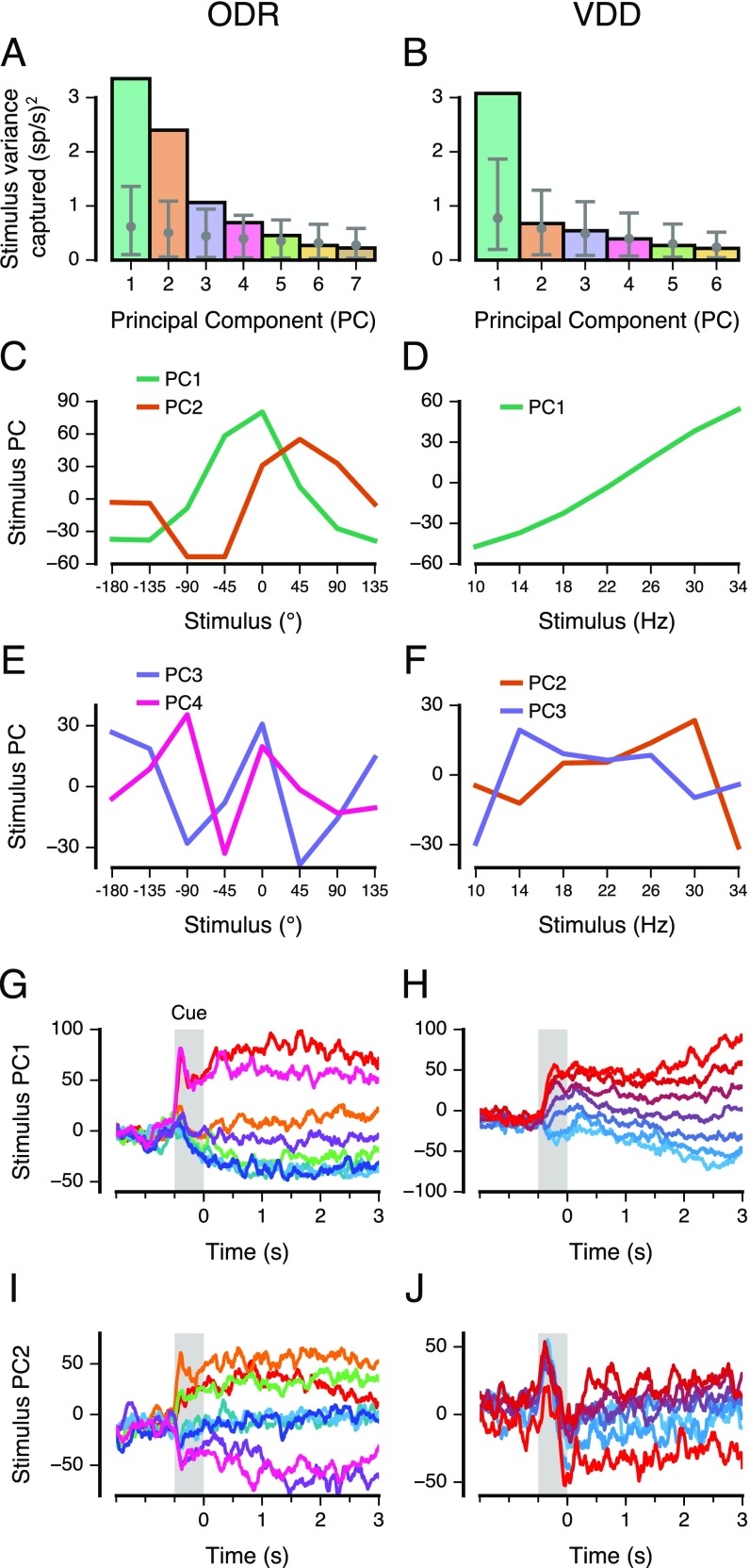
Fig. S3.
PCA of time-averaged delay activity. (A and B) Amount of stimulus variance captured by each principal axis, for time-averaged delay activity. The number of PCs is one fewer than the number of stimulus conditions. Stimulus variance captured is normalized by the number of neurons. Gray error bars show the mean and central 95% bounds, calculated through shuffling the stimulus identities of trials. For the ODR dataset, a subspace defined by the first two principal axes captures 68% of the stimulus variance. For the VDD dataset, a subspace defined by the first principal axis captures 60% of the stimulus variance. (C and D) Leading PCs, i.e., projections of the time-averaged delay activity along the leading principal axes (2 for ODR, 1 for VDD). For ODR (C), PC1 and PC2 provide quasi-sinusoidal coding of stimuli. For VDD (D), PC1 provide quasi-linear coding of stimuli. (E and F) Projections along the next two leading principal axes. (G and H) Population trajectory projected along principal axis 1, showing relative stability of stimulus coding during the delay epoch as well as in the preceding cue epoch. (I and J) Population trajectory projected along principal axis 2.

