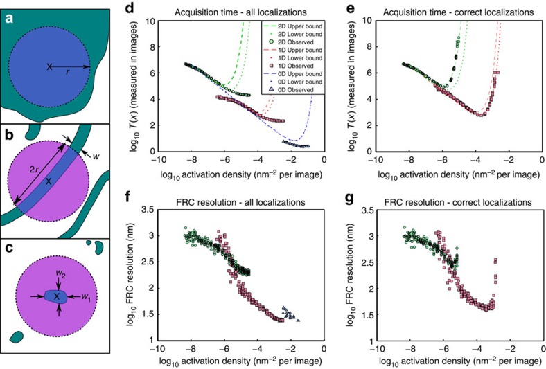
Figure 1. Effect of sample dimensionality on acquisiton time.

Demonstrates how local dimensionality changes the acquisition time needed to achieve a particular resolution. (a–c) Examples of 0D, 1D and 2D sample structures. Samples are shown in green, the exclusion area in purple and the intersection between the two in blue. The exclusion area approximately follows the pattern where is the local sample dimensionality at scale r. (a) For a 2D sample, the intersection between the exclusion zone and the sample is given by ≈πr²; (b) for a 1D sample, it is ≈2wr; (c) and for a 0D sample, ≈w₁w₂. (d,e) The theoretical and simulated values of the number of acquisition frames T(x) (to achieve a particular resolution) vary with the activation density a. Theoretical values are shown for exclusion radii of 400 nm (dashed line) and 600 nm (dotted line). The localizations returned by the fitting algorithm are displayed in d and those determined to be good fits after re-classification are shown in e. Only 2D and 1D data were reclassified; as the 0D simulated structures were very small, users were not able to reclassify accurately. An alternative approach is to evaluate the resolution for a given number of frames. This can be done with FRC (f,g). (f) The FRC resolution using all localizations returned by the analysis algorithm and (g) the FRC resolution using only those localizations classified as good.