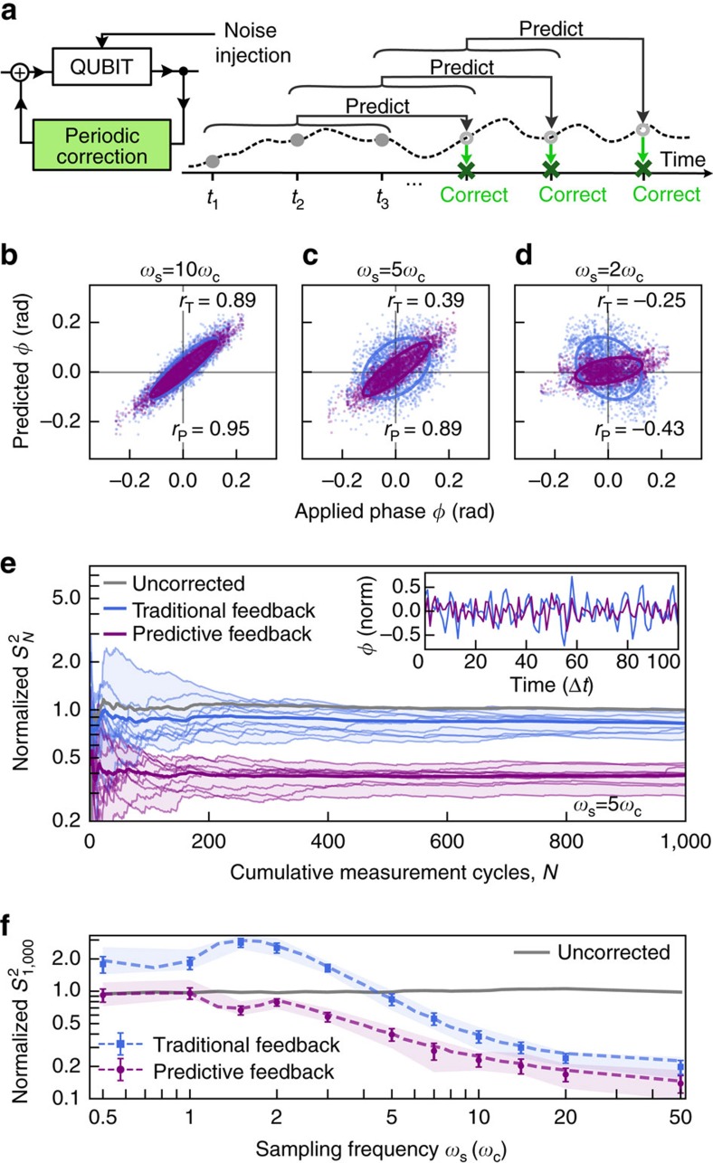
Figure 3. Experimental comparison of long-term stabilization using traditional and predictive feedback.

(a) Schematics showing the key aspects of our cyclic feedback implementation using overlapping measurements. (b–d) Demonstration of feedback accuracy for different sampling frequencies ω_s quantified in units of ω_c, presented through correlation plots (c.f. Fig. 1c) for traditional feedback (blue) and prediction (magenta). Data presented are derived from Fig. 1a. (e) Measured sample variance for various protocols as a function of the number of cycles. Data are normalized to the sample variance of the uncorrected (free-running) signal at 1,000 samples. Each line represents data taken for one particular noise realization and thick lines represent the ensemble average. The inset shows an example suppression of variance over measurement outcomes using predictive against traditional feedback (normalized to the noise amplitude). (f) Sample variance at N=1,000 as a function of sampling frequency ω_s in units of ω_c, normalized to the sample variance of the uncorrected signal. The measurement time is fixed and ω_s varied through introduction of dead time between measurements. Dotted lines display simulations and markers the measurement results averaged over ten noise realizations. Error bars represent the s.d. of the mean and the shaded areas show the maximum spread of outcomes. For fixed noise parameters varying ω_s serves as a proxy for changing the ratio of (Supplementary Discussion). Simulations and measurements in all panels use n=20.