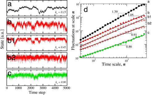
Fig. 3.

Quantification of the correlations in the state of Boolean signaling networks. As discussed, we define the state of the system as S(t) = Σ σ_i(t). We show S(t) for a system with n = 4,096 units; η = 0.1; F_i = 232; and k_e = 0.90, k_e = 0.45, and k_e = 0.15. The three values of k_e lead to quite different dynamics of the system. (a) For a small number of random links, the time correlations display trivial long-range correlations such as found for Brownian noise. (b) For an intermediate value of k_e, long-range correlations emerge and the power spectrum displays a power-law behavior, S(f) ∝ 1/f^β with β ≈ 1. b1 and b2 display the state of the system according to different definitions. In b1, the state of the system is defined as the sum of the states of a random sample comprising one-eighth of all units, whereas in b2, the state of the system is defined as the sum of the states of a block of contiguous units constituting one-eighth of the systems. Our results indicate that the evolution of a subset of the population is similar to the dynamics of the whole system. (c) For a large number of random links, k_e = 0.90, the dynamics are less correlated. (d) Estimation of temporal autocorrelations of the state of the system by the detrended fluctuation analysis method (5). We show the log–log plot of the fluctuations F(n) in the state of the system versus time scale n for the time series shown in a--c. In such a plot, a straight line indicates a power-law dependence F(n) ∝ n^α. The slope of the lines yields the scaling exponent α, which for a number of physiologic signals from free-running, healthy, and mature systems takes values close to 1 (3). The exponent α is related to the exponent β of the power spectrum of the fluctuations, S(f) ∝ 1/f^β, through the relation β = 2α - 1. The data sets have been shifted upward, and the different sets correspond (from top to bottom) to the time series shown in a–c.