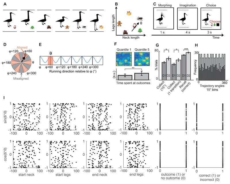
Fig. 1. Experimental design for navigation in abstract space.

(A) Subjects were trained to associate stimuli (birds) with outcomes (Christmas symbols). (B) Example trajectory in abstract space. A location in this abstract space was represented by a bird stimulus. A trajectory was equivalent to visually morphing one bird into another (Fig. 1C). The direction θ of the trajectory depended on the ratio of the rates of change of the legs and the neck (Movie S1). Subjects were not consciously aware that these associations could be organized in a continuous “bird space”. (C) Example trial corresponding to the trajectory with direction θ. (D) Trajectories can be categorized as aligned (red sectors) or misaligned (grey sectors) with the mean orientation φ of the hexagonal grid Note that φ is different for each participant (see(26) for details on how φ was calculated). Here, the direction θ is aligned with the grid. (E) fMRI markers of grid cells showing hexagonal symmetry: the signal is bigger for trajectories aligned versus those misaligned with the grid. (F) Color-coded trajectory maps illustrating time spent in each part of the environment during the “explore” task in the first (quantile1) and last parts of training (quantile5). Yellow is maximum and dark blue is 0. Barplots showing the amount of time spent at the locations/stimuli paired with outcomes in each epoch relative to the total time spent navigating (“time at outcomes” quantile1 vs quantile5, t₂₂=-3.17, ** p<0.01). (G) In the “collect” task, participants made significant improvements in training day 2 compared to training day 1: the percentage of trials with an angle error < 15° (t₃₃=2.37, * p<0.05) and with only one transition increased (t₃₃=2.55, * p<0.05). In the “recall” task, participants made significantly more correct responses in day 2 compared to day 1 (t₄₁=3.89, *** p<0.001). (H) Example data from the most commonly used schedule: even distribution of trajectory angles across all trials (light grey), outcome trials (medium grey) and non-outcome trials (dark grey). (I) Example data from the most commonly used schedule: we tested if the sin(6θ) and cos(6θ) regressors correlated with multiple confounding factors. These regressors did not correlate with the start neck, start legs, end neck and end legs lengths, whether the subject responded accurately or whether the morph passed through an outcome (all coefficients of determination R² averaged across all subjects < 0.02). (D and E are adapted by permission from Nature, Doeller et al, 2010).