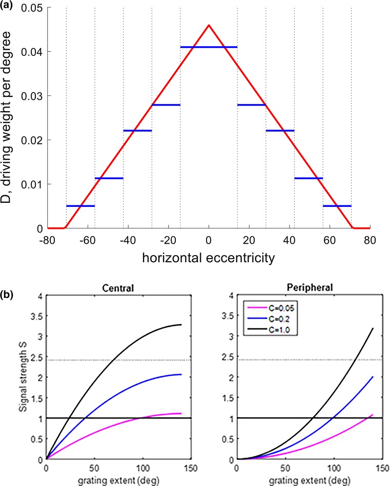
Fig. 7.

Detailed description of the model. a The modelled signal per unit degree contributing to the optomotor response, as a function of horizontal eccentricity. The sloping red lines depict the function D(x), Eq 1, with parameters fitted to Experiment 2, i.e. M = 0.046, b = 71°. The vertical dotted lines mark the boundaries of the five stimulus regions used in our model. The horizontal blue lines show the results of a more elaborate model in which the average signal contributed by each region was a free parameter, instead of being constrained to be the average value of the red line (Eq 1) in each region [fitted parameters: threshold θ = 0.90, average driving weight per degree for each patch = 1.16, 0.79, 0.62, 0.32, 0.14 (centre to periphery); cf values for linear model = 1.17, 0.91, 0.66, 0.40, 0.14]. b The modelled total signal driving the optomotor response, as a function of grating extent for central (left) and peripheral (right) locations. The curves depict the function S, Eq 2, for different stimulus sizes. The parameters were those fitted to Experiment 2, i.e. M = 0.046, b = 71°. The colours show the three different contrasts. The solid horizontal line shows the threshold, which was constrained to be equal to the SD of the noise, and the dotted line the threshold plus one SD. In our model, an optomotor response is recorded if the signal strength exceeds this threshold plus a random sample from a Gaussian with this SD