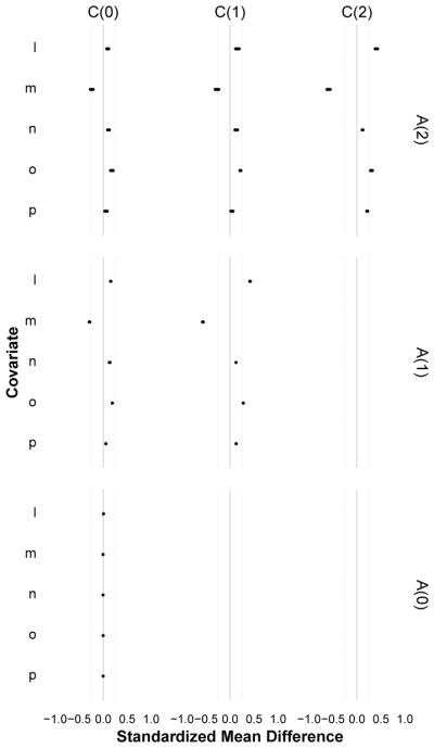
Figure 2.

A trellised covariate balance plot for Diagnostic 1 (time varying confounding), indexed by measurement times for exposure (rows) and covariates (columns). Each subplot evaluates the balance of covariates C (i.e. L,M,N,O,P) at time t − k across levels of exposure A = 1 versus A = 0 at time t, for each pattern of exposure history through time t − 1 (dots). When every dot in a horizontal plane aligns at zero, that exposure measurement is not confounded by that covariate. When this holds for all exposure measurements (across all covariates), the exposure is statistically exogenous and there is no measured time-varying confounding. In the simulated data example shown here, imbalance was largest for the most recent covariates and decayed with increasing distance between exposure and covariate times; there was no confounding at t = 0 but the pattern of confounding was the same for t = 1 and t = 2; the least balanced covariates were L (higher among the exposed) and M (higher among the unexposed), and N was the least imbalanced. Note that here, all observed exposure regimes were examined.