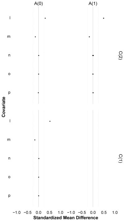
Figure 4.

A trellised covariate balance plot for Diagnostic 2a (exposure-covariate feedback), indexed by measurement times for covariates (rows) and exposure (columns). Each subplot evaluates the balance of covariates C (i.e. L,M,N,O,P) at time t across levels of exposure A = 1 versus A = 0 at time t − k, for each pattern of exposure history through time t − k − 1 (dots). For Diagnostic 2b, the plot would pertain to a specific propensity score stratum and unlike Diagnostic 2a, the dots would not represent a specific exposure history. When all the dots in a horizontal plane align at zero, the covariate measurement is independent of every prior exposure and does not contribute to exposure-covariate feedback. When this holds for every covariate measurement, there is no exposure-covariate feedback. In the simulated data example, covariate measurements for L and M were associated with previous exposures: for L the associations were strong and positive; for M they were weaker and negative. In this simulated data, any causal analysis of exposure regimes would want to consider adjusting for L and M using g-methods. Note that here, all observed exposure regimes were examined.