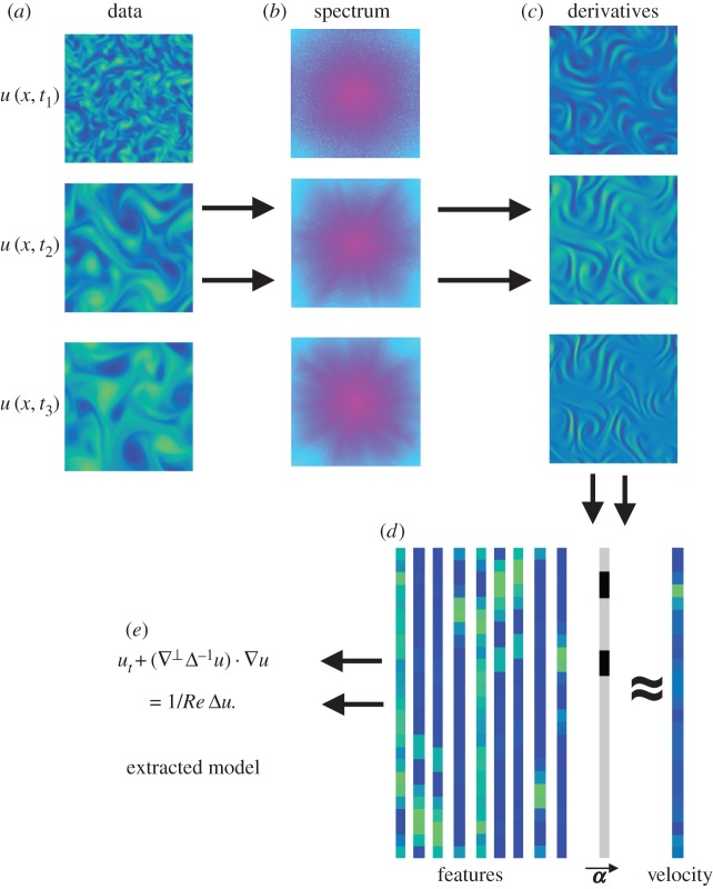
Figure 1.
Visual algorithm. The data are given as a sequence at different time stamps (a). Then, the data are converted to the Fourier domain (b) and the spatial derivatives are calculated (c). The derivatives are combined to construct features, which are then vectorized (d). An L1 optimization algorithm is used to extract the sparsity coefficients α that fit the features to the velocity. The coefficients α are unravelled to reveal the underlying model (e). (Online version in colour.)

