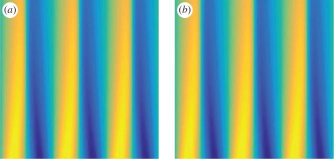
Figure 3.

Example 3.1: viscous Burgers’ equation with noise level =94.5%. The space–time dynamics are plotted to provide a qualitative comparison between the original simulation (a) and the learned dynamics (b). This shows that the parameter estimation leads to a close approximation to the original dynamics. The horizontal axis is space and the vertical axis is time. (Online version in colour.)
