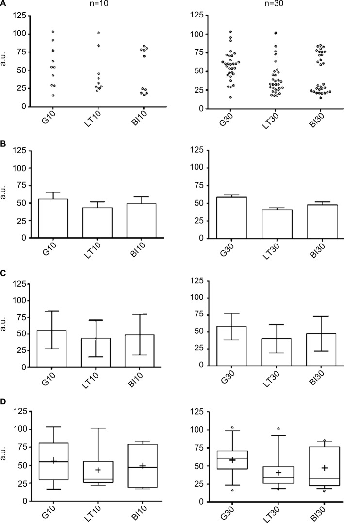
Figure 5.

Plotting views of three common distributions.

Notes: Each row contains one plotting method for three distributions (G, LT skew, and BM). Each column contains a simulated sample size of n=10 (left) or n=30 (right). The individual points showed as dot plots (A) are given for comparison visually with more common views (B–D). Bar plots with SEM (B) appear quite similar across the simulated distributions. Similarly, plotting a bard with SD (C), there is little suggestion that three different distributions are shown. When plotted using box and whiskers, we observe clues of non-Gaussian distributions; here the box is the 25–75 percentile, the line is the median, + is the mean, and the whiskers are the 2.5–97.5 percentile. In each graph, the Y-axis is in a.u.

Abbreviations: a.u., arbitrary units; BI, bimodal; G, Gaussian; LT, long tail; SD, standard deviation; SEM, standard error of the mean.