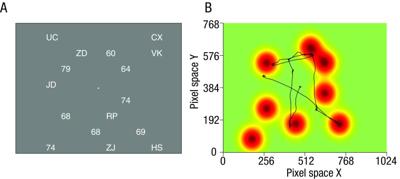
Fig. S1.

Landscape and prototypicality analysis. Our landscape analysis converts the stimulus array (A) on each trial to a topography of to-be-sampled decision values spanning the 1024 × 768 pixel space constituting the screen (B). The landscapes are created by convolving each stimulus location (i.e., the x and y coordinates of each number in pixel space) with a bivariate Gaussian basis function. Each Gaussian has an SD s and height g, with the latter reflecting some information conveyed by the stimulus. In the simplest case (B), g = 1 and s is a constant (e.g., 50 pixels). An example of such a landscape is shown in B (for the corresponding stimulus array shown in A). The estimated quality trajectory, or QT_t, which represents the total information available to the participant at any time point t, can thus be quantified as the landscape value at the current eye position (x, y) at that time point (black line in B). Across each trial, this provides a vector of values that indicate whether the participant is looking directly at a stimulus (QT_t, ∼1) or away from a stimulus (QT_t, ∼0) at each point in time following array onset. The parameter s of the Gaussian can be seen as a proxy of how much information participants can harvest around their fixation. For convenience of display, we conduct this analysis by assuming a “smooth” topography in the stimulus space. However, this is equivalent to a Gaussian filter spotlight of width s, centered at the x, y position of gaze, moving across the landscape and integrating the sum of all values under the spotlight. In this approach, the values under the spotlight are scaled by their distance to the center of the spotlight. A more in depth explanation of the landscape analysis is available in SI Methods.