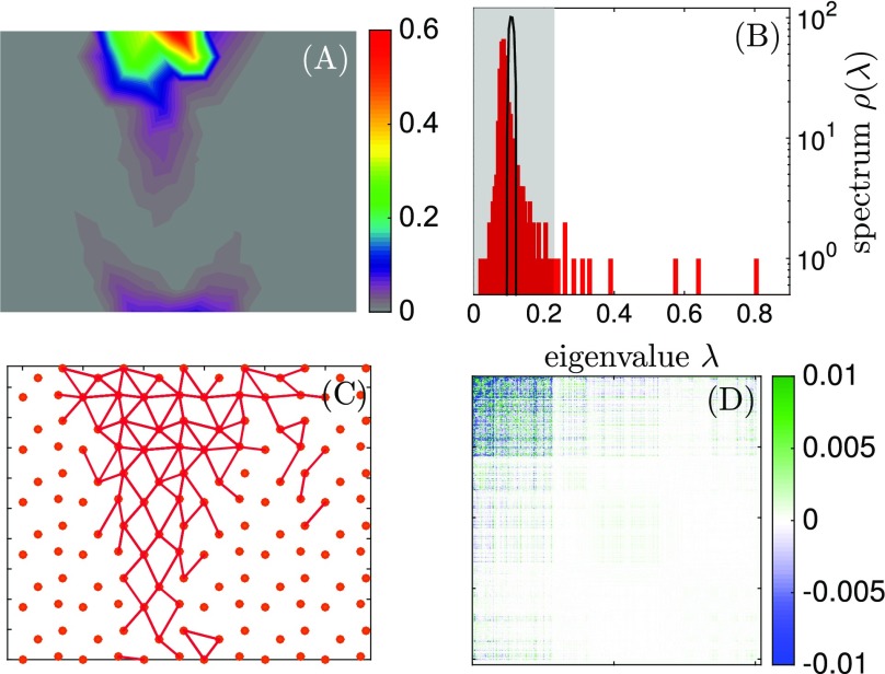
Fig. 5.

(A) Spatial distribution of conservation, as defined in Eq. 2, for $T_e=0.05$ and $z=5.0$. (B) Spectrum of eigenvalues $\rho (\lambda )$ of $C$ for the high-temperature case ($T_e=0.30$) in black and the low-temperature case ($T_e=0.05$) in red. The white region indicates which eigenvalues are used to identify the springs shown in C. (C) Springs selected using the procedure explained in Conservation and Coevolution. (D) $\stackrel{\sim }{C}$ is built using the same parameters as in C. $\stackrel{\sim }{C}$ presents a clear separation in a region where the correlations are stronger, which corresponds to the trumpet shown in C. All these images are made using $L=12$ and $z=5$.