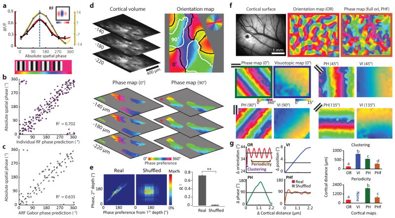
Extended Data Figure 7. Characterizing spatial phase tuning, phase column, and phase map.

a, The phase tuning from an example cell (black) and its Gaussian fit (red) compared with the phase tuning curve predicted from its receptive field structure (gray) and its Gaussian fit (yellow). Dashed line depicts the preferred phase derived from the Gaussian fit to the experimental data. b, Relation of absolute phase prediction from receptive field structure to absolute phase tuning measurement (N = 179 cells from 2 animals, P = 1.8 × 10^–18, circular regression). c, Phase preference of the orientation column is well predicted by the phase parameter of the Gabor fit to the ARF (N = 73 cortical columns from 5 animals, P = 1.7 × 10^–10, circular regression). d, Example two-photon phase maps derived from pixel tuning at three cortical depths for both horizontal and vertical orientations. e, Comparison of phase preference from different cortical depths (red asterisks in d) showing the consistence of columnar structure for spatial phase (rank-sum test for R² from circular regression, N = 36 pairs of maps at different depths from 2 animals, P = 8.2 × 10^–18). f, Large scale functional maps visualized by epi-fluorescence imaging. The phase map with full orientation coverage (right) was constructed from four individual phase maps measured independently with four orientations (0°, 45°, 90°, 135°). The phase maps for single orientations with corresponding visuotopic maps are shown separately in lower two rows. g, The statistical structure of functional maps (orientation, phase, visuotopy, and phase with 4 orientations) summarized by the relationship between the change in cortical distance and the average change in preferred feature (left). Summary comparison of clustering and periodicity of the preferred features of four functional maps from 6 animals (right). Each map exhibits distinct clustering and periodicity (N = 32 sample regions from 6 animals, Kruskal-Wallis test with post hoc using Dunn’s method, letters indicating groups with statistically significant difference, P < 0.05). All error bars indicate s.e.m.