Structural equation modeling in the context of clinical research

Abstract

Structural equation modeling (SEM) has been widely used in economics, sociology and behavioral science. However, its use in clinical medicine is quite limited, probably due to technical difficulties. Because SEM is particularly suitable for analysis of complex relationships among observed variables, it must have potential applications to clinical medicine. The article introduces basic ideas of SEM in the context of clinical medicine. A simulated dataset is employed to show how to do model specification, model fit, visualization and assessment of goodness-of-fit. The first example fits a SEM with continuous outcome variable using sem() function, and the second explores the binary outcome variable using lavaan() function.

Zhongheng Zhang, MMed.

Introduction

Structural equation modeling (SEM) combines various types of regression models to describe relationship among observed variables, aiming to provide a quantitative test of a theoretical model hypothesized by investigators (1). A set of observed variables may be used to define a construct (measurement model), and these constructs are related to each other (structural model). Constructs (latent variables or factors) are variables that are not directly observed or measured, but are defined by other observed variables. The indicators (observed or measured) are a set of variables that define or infer a construct (2). In terms of the relationship, variables can be defined as either independent or dependent variables. These terms will be referred to in the following example, which may help readers to better understand them.

The article will discuss SEM in the context of clinical research. Basic ideas and terminologies will be introduced along with the example, which may give readers a better understanding than tutorials full of mathematical details. There is a variety of R packages for SEM and its visualization, which will be discussed in the article (3).

Worked example

For the purpose of illustration, I create a dataset containing patients from intensive care unit (ICU). The research setting is employed to give readers an understanding of how to perform SEM in clinical medicine. Of note, the dataset is created by simulation technique and bears no practical interpretation. Suppose the study is designed to investigate the predictors of financial cost and mortality for ICU patients. Because there are numerous laboratory measurements being obtained for ICU patients, the complex relationships among them are difficult to disentangle. However, these laboratory measurements can be divided into broad categories. For example, c-reactive protein (crp), procalcitonin (pct) and white blood cell (wbc) are biomarkers of inflammation. Bilirubin (bil), serum creatinin (scr) and oxygen index (oxyindex) are biomarkers of organ dysfunction. However, there are no direct measurements of inflammation and organ dysfunction, thus these two are designated as latent variables. It is rational to hypothesize that inflammation causes organ dysfunction, and medical cost (cost) is increased by inflammation and organ dysfunction.

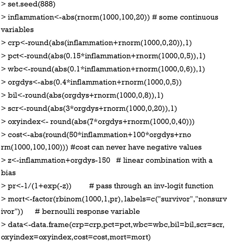
The above codes firstly set a seed [888] to allow readers to reproduce the results. Then inflammation is created as in crp scale with normal distribution. Inflammation is correlated with crp. The error term for crp has a mean of 0 and standard error of 20. Other variables are created in the same manner. All variables are forced to be positive by abs() function. Cost is determined by inflammation and organ dysfunction with an error term. Because mortality is a binary outcome, it is assumed to follow Bernoulli distribution and is created by using rbinom() function. Finally, all observed variables are combined into a data frame. Note that latent variables inflammation and orgdys are excluded because in the real world they are not observable.

Fitting the structural equation model

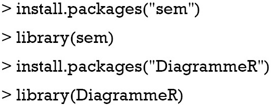
The first step in fitting the SEM is to setup environment for sem() function. Furthermore, the DiagrammeR package should be installed and loaded to the workspace for the purpose of drawing SEM diagram.

Before estimation for parameters, the structure of the model should be specified. Model specification is primarily based on subject knowledge and previous studies reporting the association between variables. The model can be specified using specifyEquations() function. Other functions such as specifyModel() can also be used. The example uses specifyEquations().

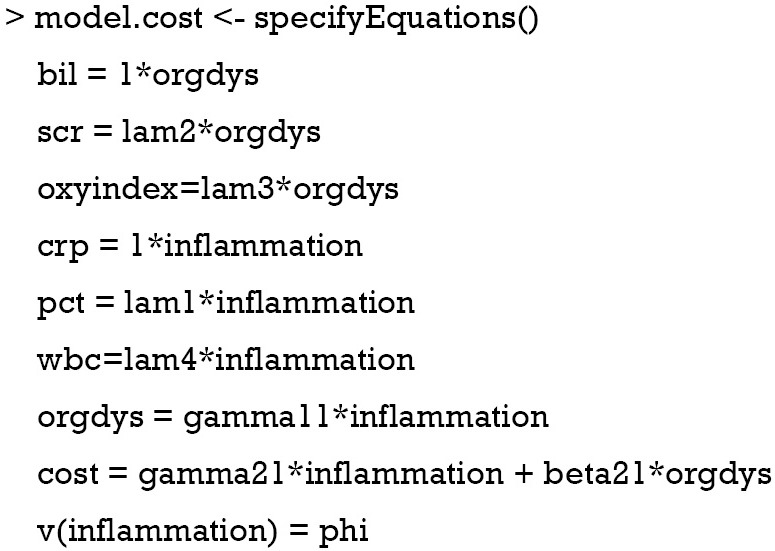
In specifyEquations(), each line specifies either a regression equation or variance or covariance. Variable on the right side of the equation is exogenous variable that it has no arrow points to it but only has arrows point out. In other terminology, exogenous variable is explanatory variable that explains changes of other variables. The left side of equation shows the parameter and endogenous variables. Endogenous variable is dependent variable that arrows point to it. The parameter is required to be estimated. If parameters are given fixed values (numeral 1 for orgdys in the example) it is treated as fixed. Otherwise, parameters are constrained if two equations use the same name for their parameters. Variances of a variable that cannot be explained by its exogenous variables are specified in the form V(variable) = parameter. Covariance of two variables are represented in the form C(variable 1, variable 2) = parameter. The symbols “v” and “c” can be in either lower- or upper-case. By default, variance for an endogenous variable will be calculated by sem() without explicitly specifying it. However, variance of an exogenous variable should be specified. In the example, inflammation is an exogenous variable and I assign phi as its variance. Next, let’s take a look at the structure of the model.

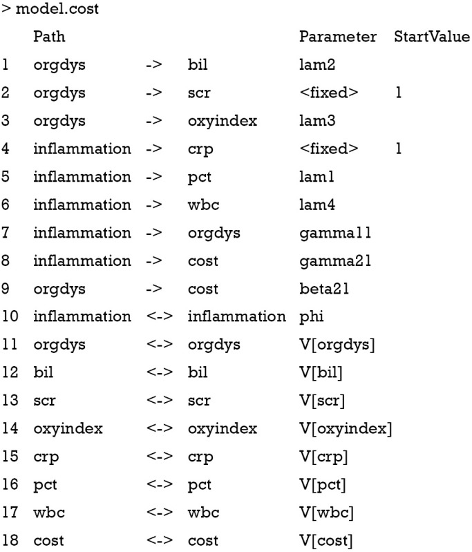
The above output displays the model in reticular action model (RAM) format via single- and double-headed arrows. Single-head arrow specifies a coefficient between variables. Double-head arrow specifies variance if two variable names are the same and covariance if corresponding variable names are different. The parameter column displays names of parameters. Because variances of endogenous variables are not explicitly specified in the example, their names take the form V[var]. The model can be fit with simple code.

Model identification

A model can be identified if there exists enough information for solution for all of the model’s parameters. Consider the equation x+2y=6, there is an infinite number of pairs of values for x and y to serve as solution to the equation. The model is underidentified because there are fewer “knowns” than “unknowns”. However, when I add another equation 3x+y=4, there is only one set of x and y satisfying both equations. Thus, the model is just identified because there are as many “knowns” as “unknowns”. In this simple example, x and y is parameters to be estimated and each equation represents an observation. When there are more parameters than observations, the model is underidentified. When there are as many parameters as observations, the model is just identified. When there are more observations than parameters (e.g., add another equation like x+y=3 to the model), the model is overidentified. The solution to overidentified model is to find a set value of x and y that the sum of squared differences between the observations (3,4) and these totals is as small as possible (4).

The SEM is comprised of structural and measurement models. In the example the measurement model describes the relationship between latent variable inflammation and observed variables crp, pct and wbc. The structural model describes the relationship between variables that we are interested in. For example, are inflammation and organ dysfunction the causes of increased financial cost in ICU patients? The order condition is the necessary requirement for a model to be identified. In order condition, the number of free parameters to be estimated must be less than or equal to the number of distinct values in matrix S. the number of distinct values in matrix S can be determined by Eq. [1]:

p×(p+1)/2 [1]

where p is the number of observed values in the model. In our example, the number of distinct values is 7×(7+1)/2=28, and the number of free parameters is 18−2=16. Note there are 18 lines in the “model.cost” output and two parameters are fixed, leaving 16 free parameters to be estimated. The model satisfies the order condition. Because there are more observations than parameters, the model is overidentified. The degree of freedom for the SEM is the difference between number of distinct values in matrix S and the number of free parameters df=28−16=12. You may want to take a look at the matrix S by the following code.

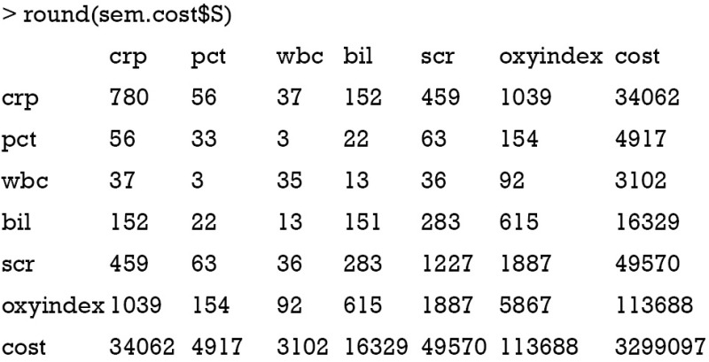
Order condition is the necessary but not the sufficient condition for model identification. Other useful conditions can aid model identification. In measurement model, the parameter is also called factor loading. The latent variable is called a construct and observed variables are indicators. Scaling the latent variable is to add a nonzero fix factor loading, which can facilitate model identification. In the example, I add a fixed factor loading 1 for observed variables crp and scr. The purpose is to fix the unit of latent measurement. The “three measure rule” states that one latent construct has at least three indicators whose errors are uncorrelated with each other. The “two measure rule” states that every latent construct is associated with at least two indicators AND every construct is correlated with at least one other construct (5-8). However, technical details of model identification is very complex and beyond the scope of this article. Next, I will use the summary() function to print the parameter estimates of the SEM, as well as statistics for model fit.

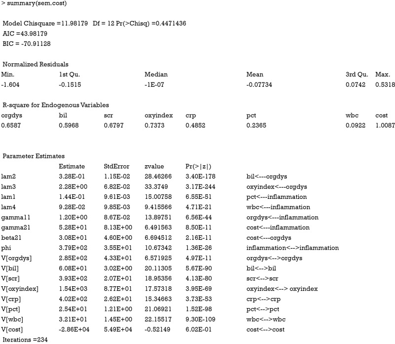
The non-significant P value of 0.45 indicates that the model cannot be rejected. Theoretically, any over-identified model can be rejected in a large sample size. Because the sample size in the example is large but there is still no evidence of under-fitting, the model can be accepted. Bayesian information criterion (BIC) is another criterion for the judgment of model fit. Negative values of BIC indicate that a model has greater support from the data than the just-identified model. The just-identified model has a BIC value of 0. BICs of alternative models can be used to compare their fits to data. It is suggested that a difference of five in BIC is a strong evidence that one model is superior to the other (9). Similarly, AIC is an alternative information criterion for model selection. Parameter estimates are of primary interests in SEM. The results show that all parameters and variances are statistically significant. That is because the data were simulated in the way the model was specified. Graphical presentation of the model can be obtained using pathDiagram() function. Note that this function requires DiagrammeR package.

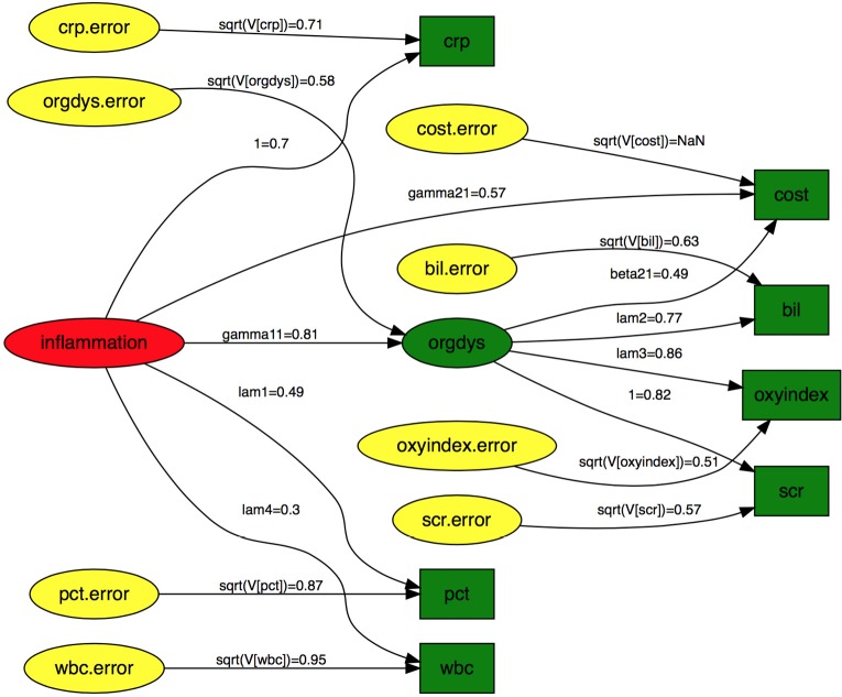
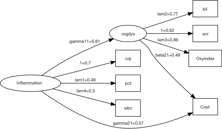
There are numerous options to customize the graphical display. In the example, I present the SEM in traditional style, which includes nodes for error variables (Figure 1). Note that latent variables and errors are represented by ellipse and observed variables are represented by rectangles. Exogenous variable is in red color. Endogenous variables are in green color and errors are in yellow color. The arrows represent parameters to be estimated with names and values displayed above each edge. One may notice that the parameter estimates displayed above the edge are not parameter estimates as shown in the summary() output. For example, gamma21, parameter for the estimate of the effect of inflammation on cost, is 0.57 in the figure. The value is 52.8 in the summary() output. Recall that I have assigned the value of 50 for this coefficient in simulation. Then how can we interpret the parameter estimates displayed in the diagram? The diagram displays standardized parameter estimates, instead of the original ones. Also note the standardized estimates for fixed parameter is not 1s. Alternatively, one may wish to draw a RAM path diagram without displaying errors (Figure 2). The default of style argument is “ram”, thus I leave it unspecified.

Figure 1.

Diagram of structural equation model in traditional style with error variables displayed. Note that latent variables and errors are represented by ellipse and observed variables are represented by rectangles. Exogenous variable is in red color. Endogenous variables are in green color and errors are in yellow color. The arrows represent parameters to be estimated with names and values displayed above each edge. crp, c-reactive protein; pct, procalcitonin; wbc, white blood cell; bil, bilirubin; scr, serum creatinin; oxyindex, oxygen index.

Figure 2.

Diagram of structural equation model in reticular action model (RAM) style, which is default to the pathDiagram() function. Note there is no error variables being displayed, making the appearance of the diagram simpler. crp, c-reactive protein; pct, procalcitonin; wbc, white blood cell; bil, bilirubin; scr, serum creatinin; oxyindex, oxygen index.

However, The pathDiagram() function provides limited options for diagram appearance. The semPaths() function shipped with semPlot package provides an alternative to draw SEM diagram after fitting the model with sem() function (10). Furthermore, this function also takes SEM object produced by other R functions such as lavaan(). Now let’s take a look at how this function works.

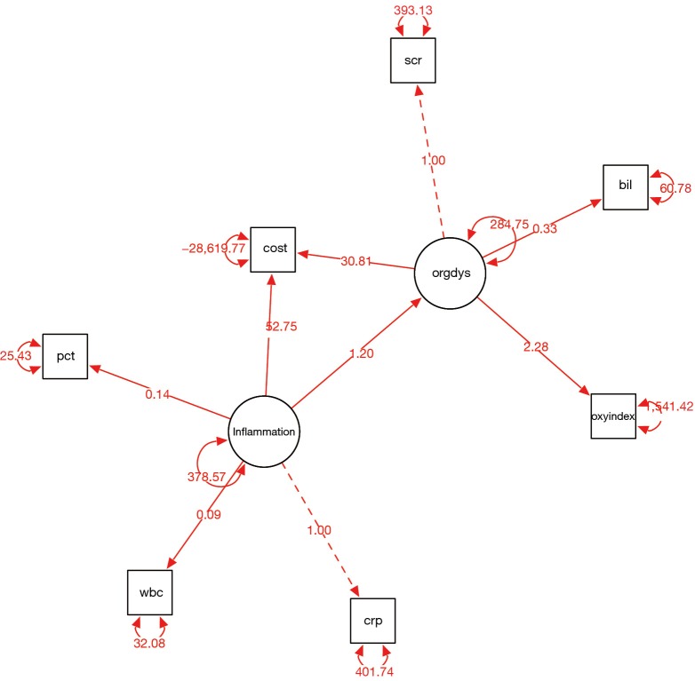
The semPaths() function takes the sem object sem.cost. The whatLabels argument specifies what the edge label should indicate. The “est” argument displays the parameter estimate in edge labels, whereas the “stand” displays the standardized parameter estimate. There are several options for the layout of the diagram. Here I use the “spring” option and the appearance is shown in Figure 3. While the solid edges represent free parameters, the dashed edges represent the fixed parameters. Other options include “tree” (the default), “circle”, “tree2” and “circle2”. The color of edges can be specified using edge.color argument.

Figure 3.

Diagram of structural equation model in spring style produced by semPaths() function. Note that parameter estimates are displayed above the edges. The values of these parameters are consistent with that produced by summary() function. crp, c-reactive protein; pct, procalcitonin; wbc, white blood cell; bil, bilirubin; scr, serum creatinin; oxyindex, oxygen index.

Interpretation of parameter estimates: direct and indirect effects

A SEM can be useful for clinicians only when its parameter interpretation is related to subject-matter knowledge. The effects() function provides estimates of the direct and indirect effects.

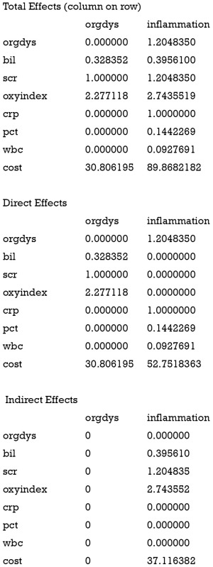
It is noted that the total effect of inflammation on cost is 89.9, which is the sum of the direct (52.8) and indirect effect (37.1). The direct effect of inflammation is its coefficient in the equation for cost, which describes the change in cost attributable to a unit change in inflammation, conditional on all other variables in the equation. This effect ignores any other simultaneous effect. The total effect of inflammation is the change in endogenous variable cost attributable to a unit change in inflammation after accounting for all the simultaneity in the system. The indirect effect acts via the latent variable organ dysfunction.

RAM

To better understand the underlying mechanisms of SEM, I would like to discuss more details on RAM model. Furthermore, some elements of RAM may help to better understand the modification index (MI) that will be discussed in the next section. The RAM model is expressed by the equation Eq. [2]:

v=Av+u [2]

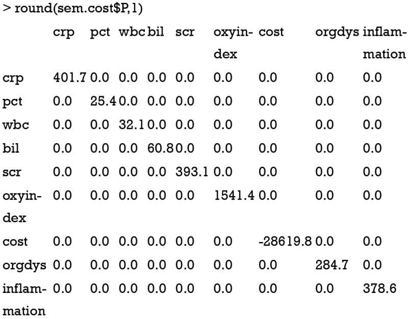
where v contains indicator variables, directly observed exogenous variables and the latent exogenous and endogenous variables. u contains directly observed exogenous variables, measurement-error variables, and structural disturbances. The matrix A contains structural coefficients and factor loadings.

As expected, the matrix A is sparse with many 0 s. Another component of RAM is the matrix P of u, which can be obtained using following code.

Model modification

A MI tells the difference in the goodness-of-fit (as measured in Chi-squares) between an existing model and a modified model in which a fixed parameter is free to be estimated. For example, if a parameter is incorrectly fixed to 1, then the test statistic for this parameter should be large. MI is a chi-square statistic with one degree of freedom; therefore a value of 3.84, which is the statistical significance threshold, requires attention. The output of modIndices() lists the five largest MI in A and P matrix (11).

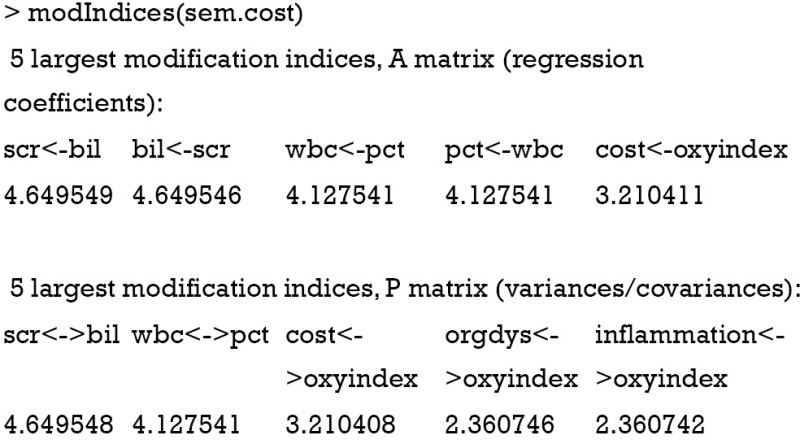
The results show that if we add an arrow from bil to scr, the chi-square of the modified model would be reduced by 4.65. The MIs in P matrix suggest the addition of covariance between observed variables. Let’s update our model under the guidance of MI. In the example, I add a covariance between scr and bil.

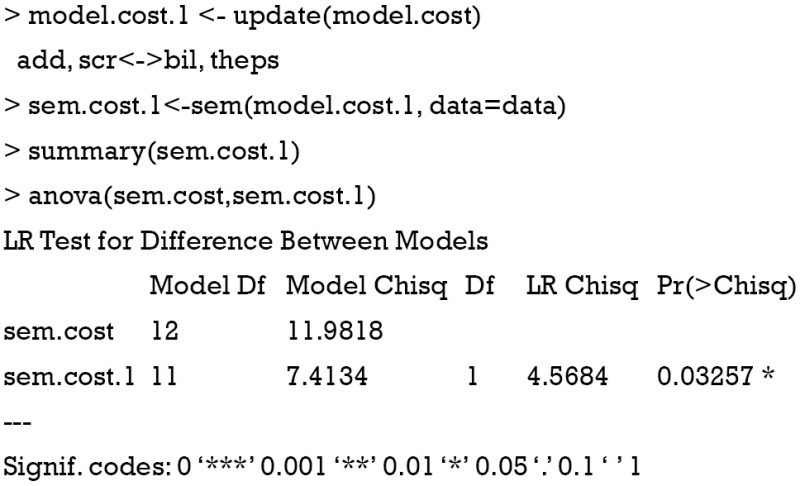
The Chi-square is 7.4 for the new model, yielding a difference of 4.6 comparing to the original model. The value is consistent with the MI of “scr<->bil”. The anova() compares the difference between the two models, and the results show that there is statistical difference between the two models. The sem.cost.1 model fits better to data than the sem.cost model.

SEM with binary endogenous variable

In clinical research, binary data are common such as mortality, gender, and occurrence of event of interest. Therefore, I would like to introduce how to model SEM with binary outcome variable using lavaan package (12). Besides, the package contains more postestimation functions that can be used to assess fitness of the model.

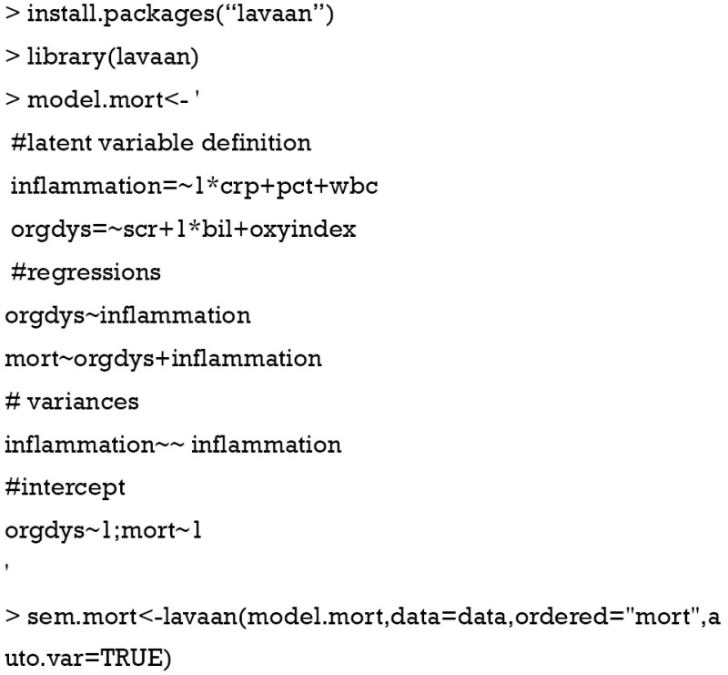
The model structure is specified with formula like expressions. It is specified as a literal string enclosed by single quotes as in the example above. The “=~” symbol links latent variable and indicators, which can be read as “is manifested by”. For the structural model, regression equations are written for each dependent variable. The regression equation is similar to that in ordinary linear regression and is specified by the “~” operator. Independent variables are linked by “+” operator on the right side of the equation. Variance and covariance are specified using “~~” operator. In the example, I set auto.var=TRUE in the lavaan() function, letting residual variances and the variances of exogenous latent variables be included in the model and set free. Intercepts are specified in special case of regression equation that there is only the number “1” on the right of the equation. Intercepts represent the mean value of a dependent variable. Because the underlying structure is known in the example, model specification can be easy. Again we can draw a SEM diagram.

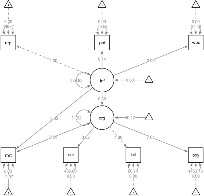
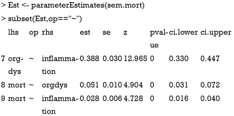
The effect of inflammation on organ dysfunction is 0.39 (Figure 4), which is consistent with the value of 0.4 that we used for simulation. The coefficients of inflammation and orgdys on mortality are 0.03 and 0.05, respectively. By exponentiation, they approximate one as specified in the simulation. The parameters of interest (parameters of structural model), as well as corresponding statistics can be examined in the following way.

Figure 4.

Diagram produced by passing a lavaan object to semPaths() function. The dependent outcome is binary. The effect of inflammation on organ dysfunction is 0.39, which is consistent with that value of 0.4 that we used for simulation. The coefficients of inflammation and orgdys on mortality are 0.03 and 0.05, respectively. By exponentiation, they approximate one as specified in the simulation. crp, c-reactive protein; pct, procalcitonin; wbc, white blood cell; bil, bilirubin; scr, serum creatinin; oxyindex, oxygen index.

Biography

Author’s introduction: Dr. Zhongheng Zhang is a fellow physician working at Sir Run-Run Shaw Hospital. He graduated from School of Medicine, Zhejiang University in 2009, receiving Master Degree. His major research interests include hemodynamic monitoring in sepsis and septic shock, delirium, and outcome study for critically ill patients. He is experienced in data management and statistical analysis by using R and STATA, big data exploration, systematic review and meta-analysis. He has published more than 50 academic papers (science citation indexed) that have been cited for over 700 times. He has been appointed as reviewer for 10 journals, including Journal of Cardiovascular Medicine, Hemodialysis International, Journal of Translational Medicine, Critical Care, International Journal of Clinical Practice, Journal of Critical Care.

References

- 1.MacCallum RC, Austin JT. Applications of structural equation modeling in psychological research. Annu Rev Psychol 2000;51:201-26. 10.1146/annurev.psych.51.1.201 [DOI] [PubMed] [Google Scholar]
- 2.Schumacker RE, Lomax RG. A Beginner's Guide to Structural Equation Modeling. 3 edition. Abingdon, OX: Routledge, 2012. [Google Scholar]
- 3.Qiu H, Song Y, Zhao T. An overview on R packages for structural equation modeling. Res J Appl Sci Eng Technol 2014;7:4182–6. 10.19026/rjaset.7.785 [DOI] [Google Scholar]
- 4.Kline RB. Principles and Practice of Structural Equation Modeling. New York: Guilford Press, 2011. [Google Scholar]
- 5.Bollen KA. Structural Equations with Latent Variables. 1 edition. Hoboken, NJ: Wiley-Interscience,1989. [Google Scholar]
- 6.Davis WR. The FC1 Rule of Identification for Confirmatory Factor Analysis: A General Sufficient Condition. Sociological Methods & Research 1993;21:403-37. 10.1177/0049124193021004001 [DOI] [Google Scholar]
- 7.Rigdon EE. Identification of structural equation models with latent variables: A review of contributions by Bekker, Merckens, and Wansbeek. Structural Equation Modeling: A Multidisciplinary Journal 1997;4:80-5. 10.1080/10705519709540061 [DOI] [Google Scholar]
- 8.Rigdon EE. A Necessary and Sufficient Identification Rule for Structural Models Estimated in Practice. Multivariate Behav Res 1995;30:359-83. 10.1207/s15327906mbr3003_4 [DOI] [PubMed] [Google Scholar]
- 9.Bollen KA, Harden JJ, Ray S, et al. BIC and Alternative Bayesian Information Criteria in the Selection of Structural Equation Models. Structural Equation Modeling: A Multidisciplinary Journal 2014;21:1-19. 10.1080/10705511.2014.856691 [DOI] [PMC free article] [PubMed] [Google Scholar]
- 10.Epskamp S. semPlot: Unified Visualizations of Structural Equation Models. Structural Equation Modeling: A Multidisciplinary Journal 2015;22:474-83. 10.1080/10705511.2014.937847 [DOI] [Google Scholar]
- 11.Fox J. TEACHER'S CORNER: Structural Equation Modeling With the sem Package in R. Structural Equation Modeling: A Multidisciplinary Journal 2006;13:465-86. 10.1207/s15328007sem1303_7 [DOI] [Google Scholar]
- 12.Rosseel Y. lavaan: An R Package for Structural Equation Modeling. Journal of Statistical Software 2012;48. [Google Scholar]