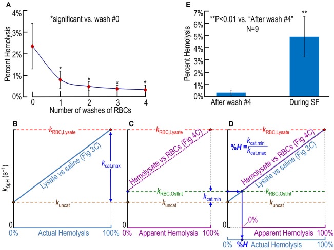
Figure 5.
Assessing RBC hemolysis. (A) Estimation of the effect of RBC washes (before stopped-flow experiments) on hemolysis, starting with whole blood containing ostensibly 100% intact RBCs. Our approaches for computing percent hemolysis before the first wash or after wash #i (i: 1–4) are described in Section Materials and Methods under “Blood collection.” (B–D) Calculation of actual percent hemolysis of ostensibly 100% intact RBCs during a SF experiment. In (B), we plot the dependence of the rate constant of pH relaxation on actual hemolysis, the latter being represented by increasing mixing ratios of RBC lysate to saline in Figure 3C. Here, kuncat represents the uncatalyzed rate constant (i.e., kΔpH without CA), kRBC, Lysate represents kΔpH in the presence of 100% lysate [with (hemoglobin) ≅ 2.5 μM], and kcat, max represents the portion of kRBC, Lysate due to the maximally catalyzed CA reaction. That is, kcat, max = kRBC, Lysate – kuncat. In (C), we plot the dependence of kΔpH on apparent hemolysis, the latter being represented increasing mixing ratios of RBC lysate to ostensibly 100% intact RBCs in Figure 4C. Here, kRBC, OstInt represents kΔpH in the presence of ostensibly 100% intact RBCs, and kcat, min represents the portion of kRBC, OstInt due to the minimally catalyzed CA reaction (i.e., that due to the small amount of CA activity released from hemolyzed RBCs in the population of ostensibly 100% intact RBCs). That is, kcat, min = kRBC, OstInt − kuncat. In (D), we overlay the plots in (B,C). The percent hemolysis (%H) of RBCs during an SF experiment is the quotient kcat, min/kcat, max. One may obtain the same answer graphically by following, first, the horizontal arrow from the y-axis and, then, the vertical arrow to %H. (E) Comparison of %H of ostensibly 100%-intact RBCs after four washes (i.e., before the SF experiment) and during SF experiments. The value for “after wash #4” in (E) is the same as for i = 4 in (A) (nine mice). The value for “During SF” in (E) is the mean for the same nine mice. For each mouse, we obtained plots that were the equivalent of those in (B) through (D), and computed a %H for that mouse. Each data point represents the mean ± SD (lower error bar not shown if it overlaps with x-axis tick mark). Differences are evaluated using the two-tailed paired student's t-test. In (A), *indicates statistical significance—after applying the Holm-Bonferroni correction—for comparisons to wash #0 of wash #1 (P = 0.0013), wash #2 (P = 0.00016), wash #3 (P = 8.4 × 10⁻⁵), and wash #4 (P = 7.2 × 10⁻⁵). None of the other comparisons in (A) yielded statistical significance. N represents the number of mice from which we obtained blood.

