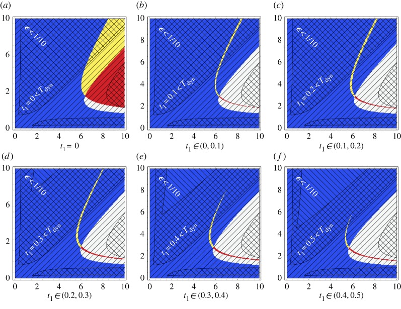
Figure 5.

Stability regions for the Gierer–Meinhardt model, as defined by the non-dimensionalization of equations (2.2) and (2.3), with parameter values d=10,ρ₁=ρ₂=ρ₃=γ=1, which are consistent with the physical scales $\hspace{0.17em}{L}_0^2/D_u=250s,\hspace{0.17em}{L}_0=5\times {10}^{-3}\hspace{0.17em}\mathrm{cm}$. Once more we have the initial condition is given by u_s(0)=u* with linear growth, φ(t)=1+rt where $r=\frac{1}{10}$. Finally, the horizontal axis in the above plots gives values of the non-dimensional kinetic parameter μ_u and similarly μ_v is given on the vertical axis. The meaning of the black diagonal lines is the same as in figure 4, as indicated by the text in white and thus the region of analytical validity is hashed. The red, white, blue and yellow regions for plot (a) are defined in exactly the same way, in terms of the stability region, $\mathcal{S}(t_0,t_0)$ and the instability region $\mathcal{U}(t_0,t_0)$, as the coloured regions in figure 4a. For plots (b) onwards the colours are analogous, but with the yellow and red regions corresponding to the set difference of the instability regions $\mathcal{U}(t_0,t_1=0.4n)\setminus \mathcal{U}(t_0,t_1=0.4(n-1))$. The yellow contribution intersects the stability region $\mathcal{S}(t_0,t_1=0.4n)$, whereas the red contribution is excluded from the stability region—the red region was an empty set in figure 4. Finally, white is the exclusion of all the other coloured regions. Note that n=1,2,3,4,5, respectively, for plots (b)–(f), with t₁=0.1n, in this figure. Thus, for instance, one can observe the evolution of Turing space for the Gierer–Meinhardt model via the yellow set differences of Turing regions in plots (b)–(f). Red online is dark grey in print (R), yellow is light grey (Y), blue is black (B) and white remains white (W). (Online version in colour.)