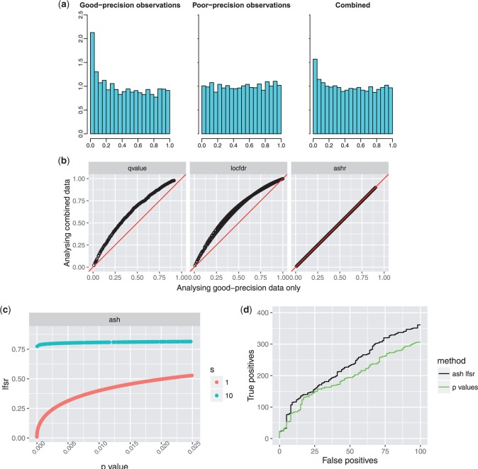
Fig. 4.
Simulations showing how, with existing methods, but not ash, poor-precision observations can contaminate signal from good-precision observations. (a) Density histograms of  values for good-precision, poor-precision, and combined observations. The combined data show less signal than the good-precision data, due to the contamination effect of the poor-precision measurements. (b) Results of different methods applied to good-precision observations only (
 -axis) and combined data (
 -axis). Each point shows the “significance” (
 values from qvalue;
  for locfdr;
  for ash) of a good-precision observation under the two different analyses. For existing methods including the poor-precision observations reduces significance of good-precision observations, whereas for ash the poor-precision observations have little effect (because they have a very flat likelihood). (c) The relationship between
  and
and  -value is different for good-precision (
 ) and low-precision (
 ) measurements: ash assigns the low-precision measurements a higher
  , effectively downweighting them. (d) Trade-off between true positives (
 ) vs false positives (
 ) as the significance threshold (
 or
or  value) is varied. By downweighting the low-precision observations ash re-orders the significance of observations, producing more true positives at a given number of false positives. It is important to note that this behaviour of ash depends on choice of
  . See Section 3.2.1 for discussion.

