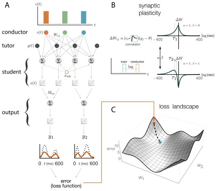
Figure 2. Schematic representation of our rate-based model.
(A) Conductor neurons fire precisely-timed bursts, similar to HVC neurons in songbirds. Conductor and tutor activities, and , provide excitation to student neurons, which integrate these inputs and respond linearly, with activity . Student neurons also receive a constant inhibitory input, . The output neurons linearly combine the activities from groups of student neurons using weights . The linearity assumptions were made for mathematical convenience but are not essential for our qualitative results (see Appendix). (B). The conductor–student synaptic weights are updated based on a plasticity rule that depends on two parameters, and , and two timescales, and (see Equation (1) and Materials and methods). The tutor signal enters this rule as a deviation from a constant threshold . The figure shows how synaptic weights change () for a student neuron that receives a tutor burst and a conductor burst separated by a short lag. Two different choices of plasticity parameters are illustrated in the case when the threshold . (C) The amount of mismatch between the system’s output and the target output is quantified using a loss (error) function. The figure sketches the loss landscape obtained by varying the synaptic weights and calculating the loss function in each case (only two of the weight axes are shown). The blue dot shows the lowest value of the loss function, corresponding to the best match between the motor output and the target, while the orange dot shows the starting point. The dashed line shows how learning would proceed in a gradient descent approach, where the weights change in the direction of steepest descent in the loss landscape.

