

Abstract
A general approach to determine orientation and distance-dependent effective intermolecular exciton transfer integrals from many-body Green’s functions theory is presented. On the basis of the GW approximation and the Bethe–Salpeter equation (BSE), a projection technique is employed to obtain the excitonic coupling by forming the expectation value of a supramolecular BSE Hamiltonian with electron–hole wave functions for excitations localized on two separated chromophores. Within this approach, accounting for the effects of coupling mediated by intermolecular charge transfer (CT) excitations is possible via perturbation theory or a reduction technique. Application to model configurations of pyrene dimers shows an accurate description of short-range exchange and long-range Coulomb interactions for the coupling of singlet and triplet excitons. Computational parameters, such as the choice of the exchange-correlation functional in the density-functional theory (DFT) calculations that underly the GW-BSE steps and the convergence with the number of included CT excitations, are scrutinized. Finally, an optimal strategy is derived for simulations of full large-scale morphologies by benchmarking various approximations using pairs of dicyanovinyl end-capped oligothiophenes (DCV5T), which are used as donor material in state-of-the-art organic solar cells.
1. Introduction
Energy transfer in molecular materials is a process in which excitation energy migrates among chromophores, e.g., a single molecule or a fragment of a larger macromolecule or molecular assembly. The control and optimization of this transfer is key to the functionality of many photoactive materials.1,2 Natural light harvesting architectures reach near 100% efficiency converting light into a chemical form (electrical energy, molecular synthesis).3,4 In contrast, the performance of many synthetic molecular devices is currently limited to significantly lower values. For instance, record power-conversion efficiencies of single-junction organic photovoltaic cells of around 11%5 still trail the estimated thermodynamic maximum,6 in part due to excitonic losses. Explicit simulations of the dynamics of excitons in complex molecular systems can be a powerful asset in revealing the interplay of electronic structure and molecular morphology on the micro- and mesoscale. Applied to a realistic representation of device materials, this knowledge will further new optimization strategies for the energy transfer processes involved. As the size of functional parts of these systems is typically on the scale of 10–100 nm, explicit ab initio treatment of the exciton dynamics is computationally intractable. Because of the disorder inherent to most organic materials as a result of material processing and thermal vibrations at room temperature, excitons tend to localize on one to a few chromophoric fragments. Localized exciton states |A⟩ can be used to define a supramolecular, tight binding like Hamiltonian as
| 1 |
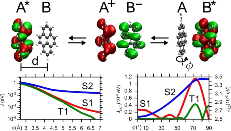
where ϵA is the associated excitation energy and JAB is the coupling between the two exciton states. JAB is sensitive to the molecular arrangement, i.e, the distance and relative orientation between chromophores, and constitutes a key ingredient in the calculation of exciton transfer rates. Depending on the type of excitation and length-scale on which the transfer occurs, different interactions and mechanisms mediate the coupling, as depicted schematically in Figure 1.
Figure 1.
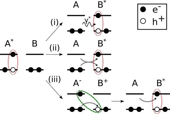
Illustration of the different pathways for exciton transfer between chromophores A and B. (i) Förster type energy transfer via exchange of a virtual photon. (ii) Dexter (charge) transfer via simultaneous hop of the electron–hole pair. (iii) CT mediated Dexter transfer via sequential hop of electron and hole.
In this paper, a dimer projection (DIPRO) method for exciton coupling based on many-body Green’s functions theory within the GW approximation and Bethe–Salpeter equation (GW-BSE)7−9 is presented. Monomer electron–hole wave functions are used as pseudo diabatic states, and a projection method is employed to express these functions in the basis of products of single-particle functions used to determine the GW-BSE Hamiltonian in a supramolecular calculation. This dimer projection procedure allows for an efficient evaluation of the direct excitonic transfer integral JAB using linear algebra methods.
The GW-BSE approach, which is traditionally more rooted in the solid-state community, has recently received increasing attention from several groups for the treatment of electronically excited states of molecular systems.10−18 One of the earlier key results is that it allows accurate description of localized (Frenkel) and bimolecular charge transfer (CT) excitons on an equal footing12,19,20 owing to its accurate inclusion of long-range Coulomb and short-range exchange interactions. A similar accuracy, in particular of the CT excitations, can typically only be achieved by time-dependent density-functional theory (TDDFT) with functionals tuned for the specific system or by higher-order wave function based approaches at significant computational cost. As has been shown by several authors, using efficient localized orbital based implementations, GW-BSE can be readily applied to molecules or clusters of molecules of technological relevance.16,17,21 Similarly, it has been realized that the use of simple self-consistent quasi-particle updates at GW level leads to improved agreement with reference energies (from experimental and/or high-level theories) as well as to a significant reduction of the notorious dependency on the DFT starting point.22 On the basis of these promising findings, a variety of development directions are currently being pursued, aiming at increased efficiency, e.g., scaling with system size via improved models for microscopic dielectric screening,23 overcoming current limitations, such as the treatment of transitions with multiple-excitation character,22 or the inclusion in hybrid quantum-mechanical molecular-mechanics (QM/MM) calculations.16−18 Specifically, here the focus is on developing a technique that allows to extend the accuracy of GW-BSE in molecule/cluster calculations to study excited state dynamics and coarsened models for supramolecular aggregates via eq 1.
Having an accurate representation of long-range Coulomb and short-range exchange interactions is of particular relevance for describing the wide range of possible excitonic coupling mechanisms, depending on the type of excitation and the involved length scales. Singlets can exhibit significant coupling even for distances exceeding 1 nm, typically estimated in the Förster picture from the interaction of the transition dipoles of the two chromophores involved in the transfer,24 see Figure 1i. On shorter length scales, higher-order multipole terms in the Coulomb coupling2 and short-range exchange effects can significantly influence the distance and orientation dependence of singlet couplings. Triplets couple exclusively via exchange interaction, which decays exponentially with chromophore distance and are therefore restricted to next neighbor transfers.25 For the exchange based contributions to singlet and triplet coupling, two distinctly different pathways need to be considered. The electron–hole pair can transfer either as an entity (Figure 1ii) or via intermediate CT states26 (see Figure 1iii). Inclusion of the CT mediated processes into an effective coupling is particularly important because they can, at short chromophore distances, contribute equally or even more than the direct process, depending on the details of the CT wave function and its energy relative to those of the localized excitons. Approximate CT wave functions have previously been constructed using, e.g., constrained DFT to study their coupling to localized excitations derived from TDDFT.27GW-BSE allows to derive both from the same Hamiltonian, and to this end, intermolecular CT excitations of types A–B+ and A+B– are constructed within GW-BSE-DIPRO as product states from the respective monomer single-particle orbitals. All the couplings between the CT excitations, as well as to the localized monomer excitons, are calculated. From these, an effective coupling JABeff is determined via a reduction technique, which maps the complete multistate system onto two effective states. Unlike previous approaches based on first-order perturbation theory, this reduction technique method is also applicable to cases with energetic resonances of CT and localized excitons.
In the following, GW-BSE-DIPRO is first applied to model configurations of pyrene dimers at various distances and orientations. As small-molecule prototype systems, these allow for a detailed analysis of the quality of the approach in application to bright and dark singlet, as well as triplet excitons. Particular emphasis is placed on the convergence of the results with respect to the number of included CT excitations as well as the differences between the perturbation and reduction techniques. After assessing the choice of the exchange-correlation functional in the density-functional theory (DFT) calculations that underly GW-BSE, optimizations of computational parameters are evaluated. For DCV5T-Me3, a dicyanovinyl end-capped oligothiophene used as donor material in state-of-the-art organic solar cells, this aims at defining a benchmark for the application of GW-BSE-DIPRO to large-scale morphologies of technologically relevant materials (Figure 2).
Figure 2.

Chemical structures of (a) pyrene and (b) DCV5T-Me3.
The paper is organized as follows: section 2 gives a concise overview of the GW-BSE formalism, including computational details, followed by a full description of the GW-BSE-DIPRO methodology. In section 3, the results of applications to pyrene and DCV5T-Me3 are presented and discussed, devising an optimal strategy for application to large-scale morphologies. A brief summary concludes the paper.
2. Methodology
2.1. Essentials of GW-BSE
Here the essentials of the GW-BSE method with relevance for the subsequent derivation of excitonic coupling are briefly summarized. For more extensive discussions, the reader is referred to the reviews in refs (8,28).
In a first step quasi-particle (QP) states representing independent electron and hole excitations are constructed based on information obtained from the Kohn–Sham (KS) energy levels of DFT:
| 2 |
In eq 2, Vext is the external potential (either of bare nuclei or pseudo atoms), VH the Hartree potential, and Vxc the exchange-correlation potential.
Within the GW approximation of many-body Green’s functions theory, as introduced by Hedin,7 excitation energies are obtained as solutions of the quasi-particle equations:
| 3 |
which contain the energy-dependent self-energy operator ∑(r,r′,E) in place of the exchange-correlation potential in eq 3. The self-energy operator is evaluated as
| 4 |
where
| 5 |
is the one-body Green’s function in quasi-particle approximation and W the dynamically screened Coulomb interaction. The latter is evaluated by first calculating the polarization P within the random-phase approximation (RPA):29−31
| 6 |
Convolution of the polarization with the bare Coulomb interaction v yields the microscopic dielectric function ϵ = 1 – vP. After determination of the inverse dielectric function ϵ–1, the result is again convoluted with the Coulomb interaction to obtain W = ϵ–1v. Because of the time-consuming evaluation of the RPA as in eq 6, it is only performed for ω = 0 (static polarization) and a generalized plasmon-pole model32 is used to extend the associated static dielectric function to the dynamic one.
In practical calculations, both G and W are determined using the ground state Kohn–Sham wave functions and energies. As DFT typically underestimates the fundamental gap EgKS, the self-energy and the resulting QP energies may typically deviate from self-consistent results by up to several 0.1 eV. Instead, an iterative procedure is employed in which a scissor shift Δn is applied to the Kohn–Sham spectrum before calculating W. The resulting quasi-particle gap Eg is determined, and from its difference to the Kohn–Sham gap, a new shift Δn+1=EgQP,n–Eg is defined. This procedure is repeated until convergence is reached. The QP energy levels are iterated in each step, implying according to eq 5 updates to the Green’s function and thus the self-energy. Note that this (limited) self-consistency treatment does not change the QP structure of eq 5 (due to satellite structures or other consequences of a self-consistent spectral shape of G(ω)).
The energetics of single-particle excitations are described with a high degree of accuracy by the quasi-particle energies.9,14,21 Optical excitations, however, cannot be treated in such an effective one-particle picture. Instead, the coupled electron–hole excitation S can be expressed as a linear combination of products of occupied (v) and empty (c) quasi-particle functions
| 7 |
AvcS is the electron–hole amplitude and can in case of singlet-to-singlet excitations be obtained by solving the generalized Bethe–Salpeter equation8,33,34 within the Tamm–Dancoff approximation28,35 (TDA)
| 8 |
D = EvirtQP – Eocc is defined via free interlevel transition energies, while Kx and Kd are the bare exchange and screened direct terms of the electron–hole interaction kernel, respectively. Finally, Ω is the transition energy of the optical excitation. For the case of triplet excitations, Kx vanishes and Ĥexc = D + Kd.
For the practical calculations in this paper, single-point Kohn–Sham calculations are performed using a modified36 version of the Gaussian03 package,37 Stuttgart/Dresden effective core potentials,38 and the associated basis sets that are augmented by additional polarization functions39 of d symmetry. For all steps of the actual GW-BSE calculations, the Gaussian-type orbital based implementation in the VOTCA package is employed.12,15,40,41 It is specifically optimized for application to molecular systems by using an auxiliary basis set to express the quantities occurring in the GW self-energy operator and the electron–hole interaction in the BSE. We include orbitals of s, p, and d symmetry with the decay constants α (in a.u.) 0.20, 0.67, and 3.0 for N and S, 0.25, 0.90, 3.0 for C, and 0.4 and 1.5 for H atoms, yielding converged excitation energies. Further technical details can be found in refs (10,42).
2.2. Excitonic Coupling Elements via GW-BSE-DIPRO
In the following, diabatic states |A⟩ and |B⟩ are approximated by monomer electron–hole wave functions, |ΦA⟩ and |ΦB⟩, as defined in eq 7, because an exact diabatization is for most systems difficult or even impossible.43 With the BSE Hamiltonian of the dimer formed by the chromophores, ĤD, one can setup an effective (2 × 2) generalized eigenvalue problem
| 9 |
with
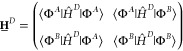 |
10 |
and
| 11 |
ci is the ith eigenvector and ϵi the corresponding eigenvalue. Because the normalized monomer states are only approximations to the diabatic states, they are not necessarily orthogonal, S ≠ 1, and JAB cannot be directly identified with the off-diagonal elements of HD. Instead, following the idea successfully established by Valeev et al. for electronic coupling,44,45 the generalized eigenvalue problem in eq 9 first needs to be transformed into a standard eigenvalue problem
| 12 |
via a Löwdin orthogonalization.46 The choice for this technique is motivated by the fact that unlike, e.g., the Schmidt orthogonalization, it treats both wave functions on an equal footing and the resulting symmetrically orthogonalized functions are the least distant in the Hilbert space from the original functions. With the orthonormalized states |Φ̃A(B)⟩, the diagonal and off-diagonal elements of H̃D can be identified with the excitation energies ϵA(B) and exciton coupling elements JAB of eq 1, respectively. It should be noted that this construction of approximate diabatic dimer states starting from monomer functions as above can be considered complementary to the approximate diabatization of adiabatic dimer states via the Boys or Mulliken–Hush scheme.47−49 While such an approach is also feasible, it comes at a higher computational cost, in particular due to the fact that solutions to eq 8 for the dimer system are required. This time-consuming step for dimers of larger molecules can be avoided using the approximation adopted here, as will be outlined in the following.
What remains is to calculate the elements of HD and S. They can be written as ⟨Φi|Ô|Φj⟩ with i ∈ A,B and Ô ={ĤD,1}. In the following, |v⟩, |α⟩, |β⟩ (|c⟩, |α′⟩, |β′⟩) are occupied (empty) single-particle orbitals of the dimer, monomer A, and monomer B, respectively. With this, the electron–hole wave functions for the localized monomer excitations (eq 7) can be written as
| 13 |
| 14 |
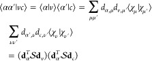
By inserting the identity I = ∑vc|vc⟩⟨vc| twice into the expression for the off-diagonal matrix elements of eq 10, and using the above definitions of |ΦA⟩ and |ΦB⟩ from eqs 13 and 14, we obtain
| 15 |
In practical calculations, Ô = ĤD is setup directly in terms of |vc⟩, so ⟨vc|ĤD|v′c′⟩ = Hvc,v′c′BSE is readily available. For Ô = 1, it holds that ⟨vc|v′c′⟩ = δvv′δcc′, yielding
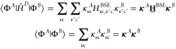 |
16 |
The quantities κA(B) are projections of the monomer electron–hole wave functions, expressed in monomer single-particles functions, onto dimer single-particle orbitals, e.g.,
| 17 |
These projections are evaluated by inserting the expansion of the respective single-particle orbitals in terms of the atomic orbital basis. When dimer and monomer calculations share the same basis set of atomic functions {|χμ⟩}, it holds that
| 18 |
| 19 |
Thus, the terms of type ⟨αα′|vc⟩ occurring in eq 17 can be rewritten as
 |
20 |
where  is the
overlap matrix of the atomic orbitals.
is the
overlap matrix of the atomic orbitals.
2.2.1. Influence of Intermolecular CT States
While the projection technique as presented above captures the coupling mechanisms depicted in Figure 1i,ii), the charge transfer state mediated mechanism (iii) is not accounted for. The aim is to include these effects, which are CT inherent and whose interactions are contained in the BSE Hamiltonian but which are not represented by the subspace spanned by |Φ̃A(B)⟩.
Intermolecular CT excitons are approximated as product states of two single-particle orbitals localized on different monomers, i.e.,
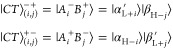 |
21 |
where αH (βH) is the highest occupied molecular orbital (HOMO) and αL (βL) is the lowest unoccupied molecular orbital (LUMO) of chromophore A(B), respectively, and i,j = 0,...,M. M is the number of additional orbitals belove (above) the HOMO (LUMO) taken into account.50 In total, a set {|CTi⟩} comprising NCT = 2(M + 1)2 CT excitations is generated according to eq 21.
As these approximate CT states are not orthogonal to the orthonormalized localized states after eq 12, each |CTi⟩ is first individually orthogonalized with respect to |Φ̃A(B)⟩
| 22 |
and then normalized via  .
.
Eq 12 then turns into a ([2 + NCT] × [2 + NCT]) eigenvalue problem with block structure of the augmented Hamiltonian:
| 23 |
where HFE = H̃D. In a final step, the subspace of CT states in eq 23 is diagonalized, i.e., solving
| 24 |
The eigenfunctions  and energies ΩiCT are used to
transform eq 23 into
an ordinary eigenvalue problem:
and energies ΩiCT are used to
transform eq 23 into
an ordinary eigenvalue problem:
| 25 |
with H̃CT = diag(ΩiCT). For the special case of M = 0, i.e., construction of two CT like excitations from the respective HOMO and LUMO single-particle orbitals, this corresponds to the (2 + 2) × (2 + 2) system
 |
26 |
2.2.2. Perturbation Theory
To obtain an effective excitonic coupling element JABeff between |Φ̃A⟩ and |Φ̃B⟩ that includes effects from coupling via intermediate CT excitations, the influence of the latter on the localized states has to be evaluated. Within first-order perturbation theory, the corrections |δΦ̃A(B)⟩ to |Φ̃A(B)⟩ due to the |CT̃i⟩ can be expressed as26,51
| 27 |
The modified coupling is then obtained to first-order in |δΦ̃A(B)⟩ as
 |
28 |
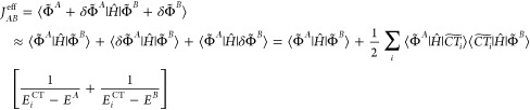
All terms required to evaluate eq 28 can be identified with elements of the Hamiltonian in eq 25: ⟨Φ̃A|Ĥ|Φ̃B⟩ is the off-diagonal element of H̃FE (i.e., the unperturbed excitonic coupling), ⟨Φ̃A|Ĥ|CT̃i⟩ are elements of H̃FE–CT, and the energies occurring in the denominator are the diagonal elements of H̃FE and H̃CT, respectively. For the example of the M = 0 case as in eq 26, the expression for the effective excitonic coupling element explicitly reads:
| 29 |
2.2.3. Reduction Method
From the structure of eq 28, it is apparent that the perturbative approach to account for the influence of CT excitations on excitonic coupling is not readily applicable to situations in which a CT excitation is energetically in, or close to, resonance with the localized excitations. Instead of going to even higher orders of perturbation theory, an alternative technique that starts from the augmented Hamiltonian of eq 25 is proposed.
The main idea is to reduce the augmented (2 + NCT) × (2 + NCT) system to an effective (2 × 2) system. In spirit similar to perturbation theory, the states forming this reduced system are expected to be close to the original states |Φ̃A(B)⟩, and consequently the effects of the intermediate CT states is mapped onto a coupling between those states. To achieve this, first eq 25 is diagonalized, yielding the eigenenergies ϵ̃i and the set of corresponding eigenvectors C~i.
From this, two elements C̃a(b) are chosen according to having the maxmium overlap with the states Φ̃A and Φ̃B, respectively. Projecting C̃a(b) onto the subspace spanned by Φ̃A and Φ̃B, followed by a Löwdin transformation, yields new orthonormalized vectors Ca(b)*.
The diagonal (2 × 2) matrix ϵ* formed with the energies ϵ̃a/b can be transformed to its nondiagonal form using the transformation matrix U = (Ca*Cb). Resulting is a reduced, effective system
| 30 |
which allows to read off the effective excitonic coupling JABeff as its diagonal elements.
To illustrate the differences and similarities between obtaining the effective coupling according to this reduction method (RM) and the perturbation theory (PT), it is convenient to consider a simplified model of the minimal system introduced in eq 26. Specifically, a symmetric system is assumed with ϵA = ϵB = ϵ, Ω1 = Ω1 = Ω, and JA(B),1(2)=JCT. Using perturbation theory, the effective coupling reads with Δϵ = Ω – ϵ
| 31 |
with the obvious resonance for Δϵ = 0. Using the reduction method yields an analytical solution
| 32 |
In the limit of Δϵ → 0, JABeff,RM remains finite. Away from the energetic resonance, i.e. Δϵ ≫JAB,JCT, it holds that
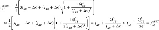 |
33 |
For more complex systems with less symmetry or M > 0, no closed form analytical expressions for JABeff,RM can be obtained. Therefore, the method is in the following employed and assessed in practical application to realistic molecular systems.
3. Results
To assess the quality of the procedures outlined in the previous section, model configurations of pyrene dimers at various distances and orientations are considered. Within the TDA of GW-BSE, pyrene exhibits energetically well separated optically inactive (S1) and active (S2) singlet as well as triplet (T1) excitations. Analysis of the excitonic couplings for these different type of excitations allows scrutinization of how well the different pathways, see Figure 1, are accounted for. The convergence of the results with respect to the number of included CT excitations, the differences between the perturbation and reduction techniques, basisset dependence, as well as the influence of the choice of the exchange-correlation functional in the density-functional theory (DFT) calculations that underly the GW-BSE steps are evaluated. Later, optimizations of computational parameters are devised using DCV5T, defining a benchmark for the application of GW-BSE-DIPRO to large-scale morphologies of technologically relevant materials.
3.1. Model Pyrene Dimers
The geometry of a single pyrene molecule was optimized on DFT level using the PBE functional52 with the 6-311G(d,p) basis set. From the this geometry, ideal π-stacked dimers with intermolecular distances ranging from 2.7 to 7 Å are constructed. GW-BSE calculations are performed for the monomers, as well as the dimer configuration (only setup of HBSE), and coupling elements determined according to the projection method.
In this configuration in which the molecules forming the dimer are related by a symmetry transformation and the energetic states of the monomers are well separated, it is also possible to obtain the effective excitonic coupling via 2Jeff = ΔΩD, where ΔΩD is the Davydov splitting of the respective monomer excitation in the dimer. To facilitate this comparison, we also perform a full GW-BSE calculation for the dimer configuration and extract the splitting from the resulting spectrum.
Figure 3 shows the distance dependence of |J| for (a) S1, (b) S2, and (c) T1 excitations obtained via GW-BSE-DIPRO with the reduction method. For all excitations, large deviations from the Davydov splitting are found when no intermediate CT states (NCT = 0) are included. At the typical π–π stacking distance of 3.5 Å, these deviations can be on the order of 1–2 orders of magnitude. For the two singlet states, the observed underestimation decreases exponentially with distance, typical for an exchange based coupling mechanism as the one mediated by charge transfer. Inclusion of CT excitations ameliorates this situation. For S2 and T1, taking only two CT excitations between the respective HOMO and LUMO states (M = 0, NCT = 2) into account practically recovers the split results. In contrast, no effect can be registered for S1. Here, an agreement with the Davydov split estimate can only be achieved for M = 1, i.e., by construction of additional CT excitations based on HOMO–1 and LUMO+1, respectively. This is due to the fact that, unlike S2 and T1, which have the main contribution from a HOMO → LUMO transition, the first singlet excitation in single pyrene is formed by a linear combination of HOMO–1 → LUMO and HOMO → LUMO+1, and the choice of M in the reduction method needs to reflect the composition of the various localized excited states. In all cases, converged exciton couplings are achieved including NCT = 50 CT excitations (M = 4). Note that for distances ≥6 Å, the coupling in S1 and T1 becomes so small that the split estimate becomes numerically inaccurate.
Figure 3.
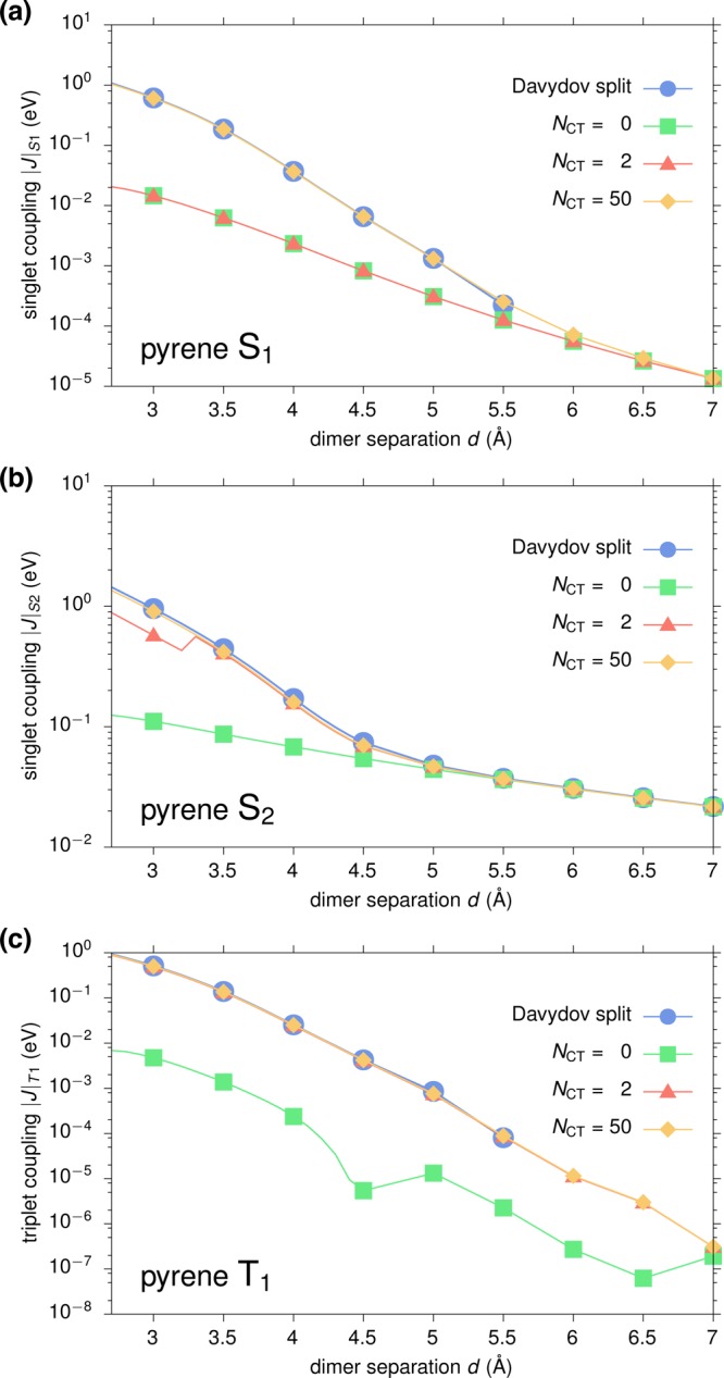
Distance dependence of excitonic couplings for (a) S1, (b) S2, and (c) T1 excitations in an ideally π-stacked pyrene dimer. Results obtained via GW-BSE-DIPRO with the reduction method for increasing numbers of included CT excitations are compared to the reference determined from the Davydov splitting in a full supermolecular calculation.
From the converged results and the Davydov splittings, it can be seen that the excitonic couplings based on GW-BSE simultaneously exhibit characteristics of short-range exchange and long-range Coulomb coupling depending on the type of excitation. For S1 (with a negligibly small transition dipole) and T1, |J| decays proportional to exp(−αd) with α(S1) ≈ 3.2 Å–1 and α(T1) ≈ 3.4 Å–1, respectively. In contrast, the optically active S2 shows an exponential decay for distances in the range of 3–4.5 Å (α(S2) ≈ 1.7 Å–1), before the effective coupling is dominated by slowly decaying Coulomb contributions.
To ascertain the quality of excitonic coupling elements obtained from GW-BSE, they are in the following compared to ones obtained from standard methods of similar complexity: time-dependent Hartree–Fock (TDHF), TDDFT/B3LYP, and configuration-interaction singles (CIS). Because the projection technique as used in GW-BSE-DIPRO is not available for those, the comparison is performed for the Davydov splittings in the ideally π-stacked dimer configurations, using the same ECP and basis set. The respective results are listed in Table 1 for dimer separations of d = 3.0–6.0 Å. At all separations, GW-BSE, TDHF, and CIS agree well for the dark S1 state. Same holds for the optically active S2. In fact, here, the data from all four methods practically agree at short and long distances, while in the intermediate region TDDFT appears to decay slightly faster. All in all, a good agreement between all four methods can be noted for singlets. For the T1 state all methods show approximately the same decay of the coupling with separation. Note, however, that TDHF calculations suffered from triplet instabilities, yielding negative excitation energies, which led to the results being discarded.53,54
Table 1. Excitonic Coupling Elements |J| from Davydov Splitting (in eV) for S1, S2, and T1 Excitations in an Ideally π-Stacked Pyrene Dimer with Varying Distance d, as Obtained by GW-BSE, TDHF, TDDFT/B3LYP, and CIS, Respectivelya.
| type | d = 3.0 Å | d = 4.0 Å | d = 5.0 Å | d = 6.0 Å |
|---|---|---|---|---|
| Davydov Split S1 | ||||
| GW-BSE | 6.13 × 10⁻¹ | 3.70 × 10⁻² | 1.53 × 10⁻³ | |
| TDHF | 6.24 × 10⁻¹ | 4.94 × 10⁻² | 2.50 × 10⁻³ | |
| TDDFT | 6.81 × 10⁻¹ | 1.08 × 10⁻¹ | 8.35 × 10⁻³ | |
| CIS | 6.41 × 10⁻¹ | 4.77 × 10⁻² | 2.50 × 10⁻³ | |
| Davydov Split S2 | ||||
| GW-BSE | 9.57 × 10⁻¹ | 1.71 × 10⁻¹ | 4.80 × 10⁻² | 2.18 × 10⁻² |
| TDHF | 8.38 × 10⁻¹ | 1.40 × 10⁻¹ | 5.11 × 10⁻² | 3.22 × 10⁻² |
| TDDFT | 6.74 × 10⁻¹ | 7.36 × 10⁻² | 3.45 × 10⁻² | 2.87 × 10⁻² |
| CIS | 8.87 × 10⁻¹ | 1.55 × 10⁻¹ | 5.60 × 10⁻² | 3.56 × 10⁻² |
| Davydov Split T1 | ||||
| GW-BSE | 5.12 × 10⁻¹ | 2.54 × 10⁻² | 8.51 × 10⁻⁴ | |
| TDDFT | 5.26 × 10⁻¹ | 3.83 × 10⁻² | 1.55 × 10⁻³ | |
| CIS | 3.97 × 10⁻¹ | 2.33 × 10⁻² | 1.70 × 10⁻³ | |
For d = 6.0 Å, the coupling in S1 and T1 becomes so small that the split estimate becomes numerically inaccurate and is therefore omitted.
In many realistic molecular aggregates, chromophores do not arrange in an ideal π-stack as assumed in the previous section. Instead, they assume relative positions and orientations characterized by shifts and rotations which are not compatible with the basic symmetry operations. Because of the asymmetry in the geometry, an estimation of coupling elements from Davydov splits is inaccurate and the use of techniques such as GW-BSE-DIPRO is indispensable. To assess the procedure for such a case, starting from the ideal π-stacking configuration with an intermolecular distance of 6.5 Å, one molecule is rotated along its long axis from 0° to 90° (see, cf., inset in Figure 4b). As for the distance dependence, the convergence of the excitonic coupling elements with respect to the number of included CT states is investigated for S1, S2, and T1. The results shown in Figure 4 generally exhibit more structure compared to the distance dependence in Figure 3 as a consequence of intricate interactions between the two π systems upon rotation. It is also evident that for rotation angles of up to approximately 50°, converged results are obtained for NCT = 50 for all excitations. At larger rotations, strong couplings are found for S1 and T1 in particular. In this region, the convergence is much slower and up to 2450 (M = 34) intermediate CT states are required. This is probably a result of the stronger and asymmetric polarization of the dimer states with respect to the monomer calculations. It should be emphasized, however, that the two chromophores approach each other very closely for those angles. At the perpendicular configuration, the minimal distance is reduced to only 3.1 Å and concomitantly strong effects and mixing of single-particle functions can be expected.
Figure 4.
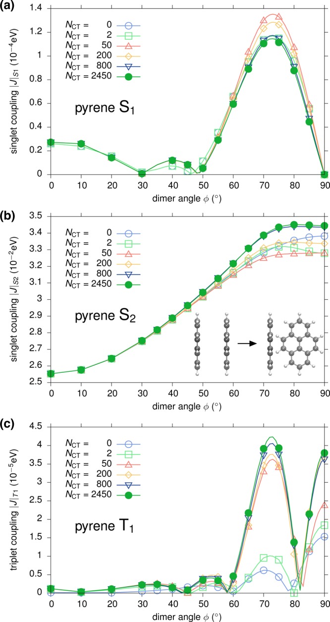
Rotational dependence of excitonic couplings for (a) S1, (b) S2, and (c) T1 excitations in a pyrene dimer. The configuration at ϕ = 0° corresponds to and ideal π-stacking at a distance of 6.5 Å. Results obtained via GW-BSE-DIPRO with the reduction method for increasing numbers of included CT excitations. Molecules have been rendered with VMD.55
To highlight the differences and similarities, distance and rotational dependence of singlet and triplet excitonic transfer integrals as obtained by the reduction method presented in this work and the perturbation theory are compared for the model pyrene configurations. In all cases, 50 CT states are included in the distance dependence and 2450 in the rotational dependence. As is apparent from Figure 5a, the distance dependence of the coupling constants for S1 and T1 shows good agreement between the approaches. Only at distances smaller than 3.5 Å perturbation theory slightly overestimates the RM results, which agree with the Davydov split estimates, cf. Figure 3. For the optically active S2 state, however, significant deviations can be observed. For an intermolecular separation of 3.5 Å, a characteristic resonance structure is found, representing a massive overestimation of the transfer integral by nearly 2 orders of magnitude. Deviations are noticeable around this typical π-stacking distance in many molecular semiconductors up to a distance of 4.5 Å. For the rotated systems, see Figure 5b; both approaches yield qualitatively similar behavior with some quantitative deviations up to a factor of 2 for the close contact structures at large rotation angles. All in all, the reduction method compares favorably with the perturbation theory approach.
Figure 5.

Comparison of the (a) distance and (b) rotation dependence of effective excitonic couplings in the pyrene model dimers, obtained with reduction method (RM) and via perturbation theory (PT), respectively. The distance dependence of both approaches as seen in (a) is nearly identical for S1 and T1 with the exception of short intermolecular distances. For the S2 couplings, large deviations are observed due to energetic resonance of localized and intermediate CT excitons. For the rotated structures (b) both approaches show similar qualitative behavior.
As mentioned in section 2, the basis set used in this work is the based on the one optimized for the use with the effective core potentials,38 which will be referred to as bsECP in the following. All results presented to this point have been obtained from calculations, in which (d,p) polarization functions of the 6-311G basis set39 have been added to form the basis bsECP(d,p). To further gauge the convergence of the reported values for the singlet and triplet exciton coupling elements with respect to the basis set choice, two basis sets with diffuse functions (bsECP(d,p)+, s shells, decay constant 0.0438 au for C, and 0.102741 au for H) and (bsECP(d,p)++, additional p shell, decay constant 0.0691 au for C) have been prepared as well. Three representative configurations of the pyrene dimers have been chosen: ideal π-stack geometries with distances 3.5 and 7.0 Å, respectively, and one at d = 5.5 Å with an additional rotation by 45°. For the latter, no results could be obtained using the bsECP(d,p)++ because of convergence issues in the underlying DFT calculation. The obtained couplings for S1, S2, and T1 excitons for these configurations are listed in Table 2. It is clear that the results are fairly independent of the choice of the basis set. Even the use of the standard bsECP without additional polarization or diffuse functions yields excitonic transfer integrals in reasonable agreement with the ones obtained by extended basis sets. This is of great significance in terms of the computational costs listed at the bottom of Table 2, from which it is obvious that the addition of diffuse functions in particular increases the calculation times dramatically. It should also be noted that this scaling of the computation time depending on the choice of basis set is exacerbated for molecules bigger than pyrene and is an important aspect to control in application to large-scale morphologies, as will be further discussed below.
Table 2. Basis Set Dependence of the Calculated Transfer Integrals |J| (in eV) for S1, S2, and T1 States in Representative Configurations of Pyrene Dimersa.
| type | bsECP | bsECP(d,p) | bsECP(d,p)+ | bsECP(d,p)++ |
|---|---|---|---|---|
| Ideal π-Stack, d = 3.5 Å | ||||
| S1 | 1.90 × 10⁻¹ | 1.85 × 10⁻¹ | 1.87 × 10⁻¹ | 1.95 × 10⁻¹ |
| S2 | 4.59 × 10⁻¹ | 4.20 × 10⁻¹ | 4.31 × 10⁻¹ | 4.53 × 10⁻¹ |
| T1 | 1.42 × 10⁻¹ | 1.37 × 10⁻¹ | 1.39 × 10⁻¹ | 1.46 × 10⁻¹ |
| Ideal π-Stack, d = 7.0 Å | ||||
| S1 | 1.86 × 10⁻⁵ | 1.35 × 10⁻⁵ | 1.33 × 10⁻⁵ | 1.32 × 10⁻⁵ |
| S2 | 2.52 × 10⁻² | 2.16 × 10⁻² | 2.19 × 10⁻² | 2.29 × 10⁻² |
| T1 | 4.18 × 10⁻⁷ | 3.08 × 10⁻⁷ | 2.47 × 10⁻⁷ | 1.62 × 10⁻⁷ |
| d = 5.5 Å, Rotation ϕ = 45° | ||||
| S1 | 3.44 × 10⁻⁴ | 4.18 × 10⁻⁴ | 4.31 × 10⁻⁴ | |
| S2 | 5.91 × 10⁻² | 4.88 × 10⁻² | 5.06 × 10⁻² | |
| T1 | 3.97 × 10⁻⁵ | 5.04 × 10⁻⁵ | 6.63 × 10⁻⁵ | |
| timings | 1.00 | 1.26 | 1.50 | 2.20 |
The average timings for the different calculations relative to the one with the smallest bsECP set are given at the bottom.
Until this point, the discussion of the GW-BSE-DIPRO approach has been limited to results obtained via GW-BSE based on DFT calculations using the semilocal PBE functional. It is known from literature that this technique can be marred by a starting point dependence, i.e., that the computed excited states depend on the quality of the underlying ground-state calculation.56 In particular, one-shot G0W0 techniques are affected by this. As a result of the iterative procedures regarding the refinement of quasi-particle energies as described in section 2 for the GW-BSE implementation used here, this problem is alleviated. To confirm this, the distance dependence of the exciton transfer integrals has been recalculated using DFT with the B3LYP hybrid functional57,58 for the pyrene dimer. The comparison to the results based on PBE as shown in Figure 6a reveals practical independence on the DFT starting point for all three types of excitations considered.
Figure 6.

Comparison of the distance dependence of exciton transfer integrals in ideally π-stacked dimers of (a) pyrene and (b) DCV5T, obtained starting from DFT calculations using PBE and B3LYP functionals, respectively. Fifty CT states have been taken into account using the reduction method.
3.2. Optimizations for Application to Large Scale Morphologies
In the following, the focus shifts to the evaluation of GW-BSE-DIPRO to chromophores of sizes typical and relevant for application in organic devices. To this end, exciton transfer integrals in an ideal stack of DCV5T molecules are investigated for the lowest energy singlet (S1, optically active) and triplet excitons (T1), respectively.
The obtained distance dependence is shown in Figure 6b, with the GW-BSE calculations being based on PBE and B3LYP DFT ground states. As for the pyrene dimer, different behavior is observed for the two excitations. The coupling of the optically active singlet states is dominated by long-range Coulomb interactions, representing Förster type coupling. In contrast, T1 shows an exponential distance dependence, as expected for a Dexter type exchange coupling. Results for the two functionals are practically identical, with a shift to slightly larger S1 couplings noticeable for PBE compared to B3LYP. This is a consequence of an approximately 9% bigger transition dipole moment resulting from the former.
The above confirms that the GW-BSE-DIPRO method used in this work is well applicable to complex molecular systems of relevant size. However, the investigation of, e.g., exciton diffusion in realistic large-scale morphologies requires the calculation of tens of thousands excitonic transfer integrals. It is therefore highly desirable to devise optimizations of the involved computational procedures. To this end, approximations on DFT, GW-BSE, and GW-BSE-DIPRO levels to decrease computation times are evaluated.
On the DFT level, it has been shown for the calculation of charge transfer integrals that it is computationally advantageous to use an initial guess for the dimer calculation formed by merging the involved densities of the monomer fragments.45 This also allows to perform only a single SCF step on the dimer instead of obtaining a fully self-consistent solution.
A possible simplification of the GW-BSE run concerns the iterative procedure used to scissor shift the Kohn–Sham spectrum before calculating W. Instead of iterating this shift for each dimer configuration, a fixed value can be predetermined, e.g., from a single representative configuration or averaging over a couple.
In Table 3, the run times and exciton transfer integrals for S1 and T1 in a DCV5T dimer separated by 3.5 Å are compared for different combinations of computational procedures. Using a fixed shift in GW-BSE saves on average 3–4 iterations, which for this system translates to reducing the runtime by approximately 4 min. The effect on the exciton couplings is negligible. Similarly, using the noSCF procedure in the DFT part has a slightly bigger effect decreasing the singlet coupling by about 1.5%. Combining both approximations cuts computation time by about 25%.
Table 3. Effect of Different Computational Parameters for DFT and GW-BSE Calculations on Run Times and Exciton Transfer Integrals for S1 and T1 in a DCV5T Dimer Separated by 3.5 Åa.
| DFT@PBE | GW-BSE | time [min:s] | |J|S1 [eV] | |J|T1 [eV] |
|---|---|---|---|---|
| SCF | iterate | 44:50 | 0.5354 | 0.1709 |
| SCF | fixed | 40:28 | 0.5355 | 0.1710 |
| noSCF | iterate | 37:51 | 0.5277 | 0.1721 |
| noSCF | fixed | 33:40 | 0.5278 | 0.1721 |
Calculations were performed using four threads on a i5-4690 CPU @3.50 GHz. The value of 0.22 Ryd for the fixed shift runs was taken from the result of the iterative procedure at 3 Å.
Additionally, the distance dependence of triplet and singlet couplings in DCV5T has been calculated for all four options given in Table 3. The results shown in Figure 7 underline that the choice of noSCF and fixed shift does not lead to larger deviations even at greater intermolecular separations. Even though this choice reduces the computational time by 25% compared to using fully self-consistent procedures on all levels, the remaining absolute time is still substantial. In particular, the slow distance decay of couplings for optically active singlets implies the necessity to determine transfer integrals for a number of chromophore dimers that is intractable for any first-principles based technique such as GW-BSE-DIPRO.
Figure 7.

Comparison of the effect of different approximations on the distance dependence of triplet (a) and singlet (b) couplings in DCV5T. Inset in (b) shows additionally estimates from transition partial charges and transition dipole interactions for very long distances.
The setup of the dimer GW-BSE Hamiltonian matrix takes up a significant amount of the total computer time when applied to larger molecules. As stated in section 2, we have so far considered all nocc occupied and as many virtual single-particle levels in the construction of the product basis for the dimer. With nocc = 186 for DCV5T, this corresponds to a matrix of dimension 34569. Naturally, calculations can be accelerated by reducing the number of single particle states taken into account in this step. Using several values of the factor f to set the range single particle states considered to [nocc(1 – f):nocc(1 + f)], the relative reduction in computational time and relative deviation of singlet couplings is evaluated. As depicted in Figure 8, reducing f to 0.5 approximately halves the computational cost, while only a 8% decrease in accuracy is observed.
Figure 8.
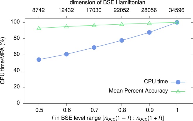
Relative reduction of computation time of the GW-BSE calculation (excluding the DFT part) for the DCV5T singlet coupling. Couplings were calculated for five distances and the relative errors with respect to the high dimension BSE result averaged.
Furthermore, it can be assumed that beyond some distance, the long-ranged couplings are given as classical Coulomb interactions of transitions densities of the constituent chromophores. It is convenient to map the full transition density to a set of atomic partial charges that reproduces its electrostatic potential.59,60 Such a classical model allows the computation of many thousands excitonic transfer integrals per minute. As can be seen in Figure 7b, the results from this TrESP approach agree well with the GW-BSE-DIPRO couplings beyond a separation of 5 Å, a typical distance at which intermolecular exchange effects can be expected to be negligible relative to the Coulomb interactions of large transition densities. The inset shows a comparison between classical interactions of transition charges with those of transition dipoles (TrDip), a coarser and often employed representation of transition densities. At a distance of 5 Å, the dipole coupling overestimates the TrESP and GW-BSE-DIPRO results by 1 order of magnitude. Practical agreement can only be observed for separations larger than 60 Å, casting doubts about the use of the TrDip approximation for intermediate distances.
4. Summary
In this paper, a general approach to determine orientation and distance-dependent effective intermolecular exciton transfer integrals from many-body Green’s functions theory within the GW approximation and the Bethe–Salpeter equation (BSE) has been derived. A projection technique is employed to obtain the excitonic coupling by forming the expectation value of a supramolecular BSE Hamiltonian with electron–hole wave functions for excitations localized on two separated chromophores. Within this approach effects of coupling mediated by intermolecular charge transfer (CT) excitations are accounted for via a reduction technique that proves to be applicable to situation in which conventional perturbative approaches break down.
Application to model dimers reveals an accurate description of short-range exchange and long-range Coulomb interactions for the coupling of singlet and triplet excitons by this GW-BSE-DIPRO technique. An optimal strategy for simulations of full large-scale morphologies includes a combination of loosening of self-consistency parameters, reduction of the active space in GW-BSE, and, for optically active singlets, a change to classical transition density-based interaction models at larger distances. All developed methods are available within VOTCA software package.41
Acknowledgments
This work was partially supported by Deutsche Forschungsgemeinschaft (DFG) program IRTG 1404. The authors are grateful to Raffaello Potestio, Behnaz Bagheri, Pranav Madhikar, Yuriy Khalak, and Mikko Karttunen for a critical reading of the manuscript.
The authors declare no competing financial interest.
References
- Mikhnenko O. V.; Blom P. W. M.; Nguyen T.-Q. Energy Environ. Sci. 2015, 8, 1867–1888. 10.1039/C5EE00925A. [DOI] [Google Scholar]
- Athanasopoulos S.; Hennebicq E.; Beljonne D.; Walker A. B. J. Phys. Chem. C 2008, 112, 11532–11538. 10.1021/jp802704z. [DOI] [Google Scholar]
- Cheng Y.-C.; Fleming G. R. Annu. Rev. Phys. Chem. 2009, 60, 241–262. 10.1146/annurev.physchem.040808.090259. [DOI] [PubMed] [Google Scholar]
- Sener M. K.; Jolley C.; Ben-Shem A.; Fromme P.; Nelson N.; Croce R.; Schulten K. Biophys. J. 2005, 89, 1630–1642. 10.1529/biophysj.105.066464. [DOI] [PMC free article] [PubMed] [Google Scholar]
- Green M. A.; Emery K.; Hishikawa Y.; Warta W.; Dunlop E. D. Prog. Photovoltaics 2015, 23, 1–9. 10.1002/pip.2573. [DOI] [Google Scholar]
- Gruber M.; Wagner J.; Klein K.; Hörmann U.; Opitz A.; Stutzmann M.; Brütting W. Adv. Energy Mater. 2012, 2, 1100–1108. 10.1002/aenm.201200077. [DOI] [Google Scholar]
- Hedin L. Phys. Rev. 1965, 139, A796–A823. 10.1103/PhysRev.139.A796. [DOI] [Google Scholar]
- Onida G.; Reining L.; Rubio A. Rev. Mod. Phys. 2002, 74, 601. 10.1103/RevModPhys.74.601. [DOI] [Google Scholar]
- Rohlfing M. Int. J. Quantum Chem. 2000, 80, 807–815. . [DOI] [Google Scholar]
- Ma Y.; Rohlfing M.; Molteni C. Phys. Rev. B: Condens. Matter Mater. Phys. 2009, 80, 241405. 10.1103/PhysRevB.80.241405. [DOI] [Google Scholar]
- Blase X.; Attaccalite C.; Olevano V. Phys. Rev. B: Condens. Matter Mater. Phys. 2011, 83, 115103. 10.1103/PhysRevB.83.115103. [DOI] [Google Scholar]
- Baumeier B.; Andrienko D.; Rohlfing M. J. Chem. Theory Comput. 2012, 8, 2790–2795. 10.1021/ct300311x. [DOI] [PubMed] [Google Scholar]
- Marom N.; Caruso F.; Ren X.; Hofmann O. T.; Körzdörfer T.; Chelikowsky J. R.; Rubio A.; Scheffler M.; Rinke P. Phys. Rev. B: Condens. Matter Mater. Phys. 2012, 86, 245127. 10.1103/PhysRevB.86.245127. [DOI] [Google Scholar]
- van Setten M. J.; Weigend F.; Evers F. J. Chem. Theory Comput. 2013, 9, 232–246. 10.1021/ct300648t. [DOI] [PubMed] [Google Scholar]
- Baumeier B.; Andrienko D.; Ma Y.; Rohlfing M. J. Chem. Theory Comput. 2012, 8, 997–1002. 10.1021/ct2008999. [DOI] [PubMed] [Google Scholar]
- Baumeier B.; Rohlfing M.; Andrienko D. J. Chem. Theory Comput. 2014, 10, 3104–3110. 10.1021/ct500479f. [DOI] [PubMed] [Google Scholar]
- Bagheri B.; Karttunen M.; Baumeier B. Eur. Phys. J.: Spec. Top. 2016, 225, 1743–1756. 10.1140/epjst/e2016-60144-5. [DOI] [Google Scholar]
- Bagheri B.; Baumeier B.; Karttunen M. Phys. Chem. Chem. Phys. 2016, 18, 30297–30304. 10.1039/C6CP02944B. [DOI] [PubMed] [Google Scholar]
- Blase X.; Attaccalite C. Appl. Phys. Lett. 2011, 99, 171909. 10.1063/1.3655352. [DOI] [Google Scholar]
- Sharifzadeh S.; Darancet P.; Kronik L.; Neaton J. B. J. Phys. Chem. Lett. 2013, 4, 2197–2201. 10.1021/jz401069f. [DOI] [Google Scholar]
- Faber C.; Boulanger P.; Attaccalite C.; Duchemin I.; Blase X. Philos. Trans. R. Soc., A 2014, 372, 20130271. 10.1098/rsta.2013.0271. [DOI] [PubMed] [Google Scholar]
- Jacquemin D.; Duchemin I.; Blase X. J. Chem. Theory Comput. 2015, 11, 3290–3304. 10.1021/acs.jctc.5b00304. [DOI] [PMC free article] [PubMed] [Google Scholar]
- Rohlfing M. Phys. Rev. B: Condens. Matter Mater. Phys. 2010, 82, 205127. 10.1103/PhysRevB.82.205127. [DOI] [Google Scholar]
- Förster T. Ann. Phys. 1948, 437, 55–75. 10.1002/andp.19484370105. [DOI] [Google Scholar]
- You Z.-Q.; Hsu C.-P. J. Chem. Phys. 2010, 133, 074105. 10.1063/1.3467882. [DOI] [PubMed] [Google Scholar]
- Harcourt R. D.; Scholes G. D.; Ghiggino K. P. J. Chem. Phys. 1994, 101, 10521. 10.1063/1.467869. [DOI] [Google Scholar]
- Difley S.; van Voorhis T. J. Chem. Theory Comput. 2011, 7, 594–601. 10.1021/ct100508y. [DOI] [PubMed] [Google Scholar]
- Bechstedt F.Many-Body Approach to Electronic Excitations; Springer Series in Solid-State Sciences; Springer: Berlin, Heidelberg, 2015; Vol. 181. [Google Scholar]
- Hybertsen M. S.; Louie S. G. Phys. Rev. Lett. 1985, 55, 1418–1421. 10.1103/PhysRevLett.55.1418. [DOI] [PubMed] [Google Scholar]
- Godby R. W.; Schlüter M.; Sham L. J. Phys. Rev. Lett. 1986, 56, 2415–2418. 10.1103/PhysRevLett.56.2415. [DOI] [PubMed] [Google Scholar]
- Rohlfing M.; Krüger P.; Pollmann J. Phys. Rev. Lett. 1995, 75, 3489–3492. 10.1103/PhysRevLett.75.3489. [DOI] [PubMed] [Google Scholar]
- von der Linden W.; Horsch P. Phys. Rev. B: Condens. Matter Mater. Phys. 1988, 37, 8351–8362. 10.1103/PhysRevB.37.8351. [DOI] [PubMed] [Google Scholar]
- Hanke W.; Sham L. J. Phys. Rev. B: Condens. Matter Mater. Phys. 1980, 21, 4656–4673. 10.1103/PhysRevB.21.4656. [DOI] [Google Scholar]
- Onida G.; Reining L.; Godby R. W.; del Sole R.; Andreoni W. Phys. Rev. Lett. 1995, 75, 818–821. 10.1103/PhysRevLett.75.818. [DOI] [PubMed] [Google Scholar]
- For typical donor molecules used in organic solar cells, we showed that the use of the TDA overestimates π–π transition energies by 0.2 eV but yields correct character of the excitations.15
- The source code of Gaussian03 was modified to output the matrix elements of the exchange-correlation potential in the atomic orbital basis, needed to calculate the matrix ⟨n |Vxc |m⟩, where |n⟩ and |m⟩ are Kohn–Sham wave functions, as input for the GW-BSE steps.
- Frisch M. J.; Jaramillo J.; Gomperts R.; Stratmann R. E.; Yazyev O.; Austin A. J.; Cammi R.; Pomelli C.; Ochterski J. W.; Ayala P. Y.; Morokuma K.; Voth G. A.; Salvador P.; Dannenberg J. J.; Zakrzewski V. G.; Dapprich S.; Daniels A. D.; Strain M. C.; Farkas O.; Malick D. K.; Rabuck A. D.; Raghavachari K.; Foresman J. B.; Ortiz J. V.; Cui Q.; Baboul A. G.; Clifford S.; Cioslowski J.; Stefanov B. B.; Liu G.; Liashenko A.; Piskorz P.; Komaromi I.; Martin R. L.; Fox D. J.; Keith T.; Al-Laham M. A.; Peng C. Y.; Nanayakkara A.; Challacombe M.; Gill P. M. W.; Johnson B.; Chen W.; Wong M. W.; Gonzalez C.; Pople J. A.. Gaussian 03, revision C.02; Gaussian Inc.: Wallingford, CT, 2004.
- Bergner A.; Dolg M.; Kuchle W.; Stoll H.; Preuss H. Mol. Phys. 1993, 80, 1431–1441. 10.1080/00268979300103121. [DOI] [Google Scholar]
- Krishnan R.; Binkley J. S.; Seeger R.; Pople J. A. J. Chem. Phys. 1980, 72, 650. 10.1063/1.438955. [DOI] [Google Scholar]
- Rühle V.; Lukyanov A.; May F.; Schrader M.; Vehoff T.; Kirkpatrick J.; Baumeier B.; Andrienko D. J. Chem. Theory Comput. 2011, 7, 3335–3345. 10.1021/ct200388s. [DOI] [PMC free article] [PubMed] [Google Scholar]
- Available on www.votca.org.
- Ma Y.; Rohlfing M.; Molteni C. J. Chem. Theory Comput. 2010, 6, 257–265. 10.1021/ct900528h. [DOI] [PubMed] [Google Scholar]
- Mead C. A.; Truhlar D. G. J. Chem. Phys. 1982, 77, 6090–6098. 10.1063/1.443853. [DOI] [Google Scholar]
- Valeev E. F.; Coropceanu V.; da Silva Filho D. A.; Salman S.; Brédas J.-L. J. Am. Chem. Soc. 2006, 128, 9882–9886. 10.1021/ja061827h. [DOI] [PubMed] [Google Scholar]
- Baumeier B.; Kirkpatrick J.; Andrienko D. Phys. Chem. Chem. Phys. 2010, 12, 11103–11113. 10.1039/c002337j. [DOI] [PubMed] [Google Scholar]
- Löwdin P.-O. J. Chem. Phys. 1950, 18, 365–375. 10.1063/1.1747632. [DOI] [Google Scholar]
- Hsu C.-P. Acc. Chem. Res. 2009, 42, 509–518. 10.1021/ar800153f. [DOI] [PubMed] [Google Scholar]
- Hsu C.-P.; You Z.-Q.; Chen H.-C. J. Phys. Chem. C 2008, 112, 1204–1212. 10.1021/jp076512i. [DOI] [Google Scholar]
- Voityuk A. A. J. Phys. Chem. C 2014, 118, 1478–1483. 10.1021/jp410802d. [DOI] [Google Scholar]
- For the sake of a compact presentation, M is chosen to be the same for both occupied and unoccupied levels of both molecules forming the dimer. In the actual implementation, these numbers can be chosen independently to account for potentially different densities of state.
- Lunkenheimer B.Simulationen zur Exzitonendiffusion in organischen Halbleitern. Ph.D. Thesis. Universitätsbibliothek, Mainz, 2014. [Google Scholar]
- Perdew J. P.; Burke K.; Ernzerhof M. Phys. Rev. Lett. 1996, 77, 3865–3868. 10.1103/PhysRevLett.77.3865. [DOI] [PubMed] [Google Scholar]
- Peach M. J. G.; Williamson M. J.; Tozer D. J. J. Chem. Theory Comput. 2011, 7, 3578–3585. 10.1021/ct200651r. [DOI] [PubMed] [Google Scholar]
- Cordova F.; Doriol L. J.; Ipatov A.; Casida M. E.; Filippi C.; Vela A. J. Chem. Phys. 2007, 127, 164111. 10.1063/1.2786997. [DOI] [PubMed] [Google Scholar]
- Humphrey W.; Dalke A.; Schulten K. J. Mol. Graphics 1996, 14, 33–38. 10.1016/0263-7855(96)00018-5. [DOI] [PubMed] [Google Scholar]
- Bruneval F.; Marques M. A. L. J. Chem. Theory Comput. 2013, 9, 324–329. 10.1021/ct300835h. [DOI] [PubMed] [Google Scholar]
- Becke A. D. J. Chem. Phys. 1993, 98, 5648. 10.1063/1.464913. [DOI] [Google Scholar]
- Stephens P. J.; Devlin F. J.; Chabalowski C. F.; Frisch M. J. J. Phys. Chem. 1994, 98, 11623–11627. 10.1021/j100096a001. [DOI] [Google Scholar]
- Kistler K. A.; Spano F. C.; Matsika S. J. Phys. Chem. B 2013, 117, 2032–2044. 10.1021/jp310603z. [DOI] [PubMed] [Google Scholar]
- Chang J. C. J. Chem. Phys. 1999, 67, 3901–3909. 10.1063/1.435427. [DOI] [Google Scholar]