Fig. 5.

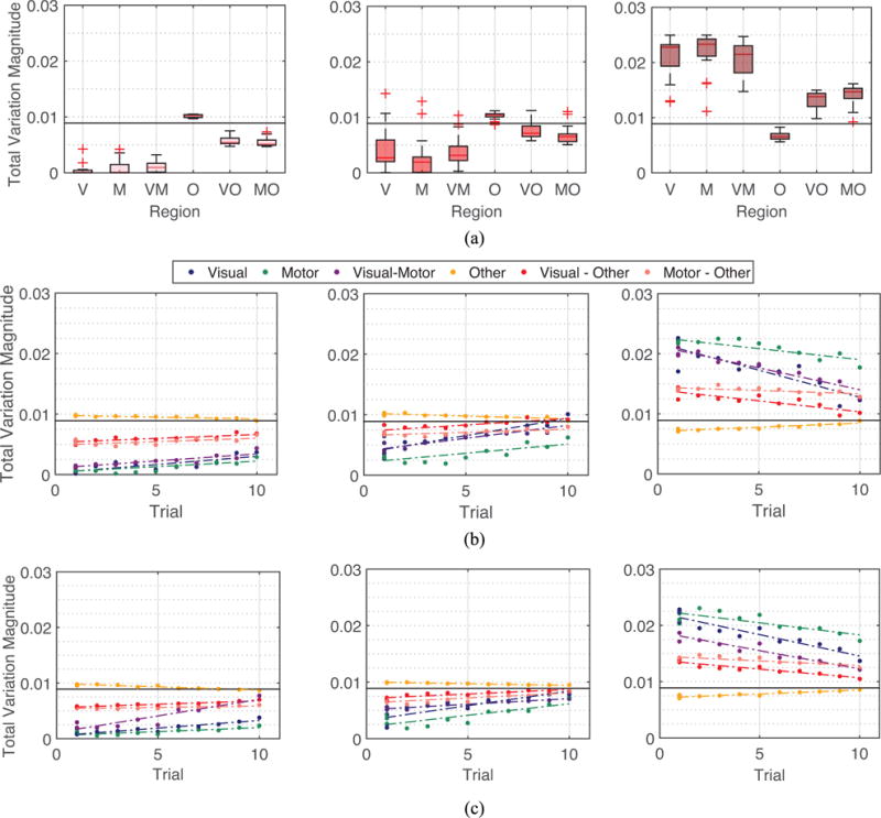
Spectral property of brain networks in the 6 week experiment. (a) Left: Averaged total variation of eigenvectors v_k for 6 different types of connections of the brain averaged across all eigenvectors associated with low graph frequencies ${\mathbf{v}}_k\in {\left\{{\mathbf{v}}_k\right\}}_{k=0}^{K_{\mathrm{L}}-1}$, across all participants and scan sessions. Middle: Across all eigenvectors associated with mid-range graph frequencies ${\mathbf{v}}_k\in {\left\{{\mathbf{v}}_k\right\}}_{k=K_{\mathrm{L}}}^{K_{\mathrm{L}}+K_{\mathrm{M}}-1}$. Right: Across all eigenvectors with high graph frequencies ${\mathbf{v}}_k\in {\left\{{\mathbf{v}}_k\right\}}_{k=K_{\mathrm{L}}+K_{\mathrm{M}}}^{n-1}$. (b) Median total variations of brain networks across participants of different scanning sessions and different sequence types with respect to the level of exposure of participants to the sequence type at the scanning session. Relationship between training duration, intensity, and depth is summarized in Fig. 1. Value of 1 on the x-axis in the figures refers to minimum exposure to sequences (all 3 sequence types of the first session), and value of 10 on the x-axis denotes the maximum exposure to sequences (EXT sequence types of the fourth session). An association between spectral property of brain networks and the level of exposure is clearly observed (average correlation coefficient 0.8164). (c) Median total variations evaluated upon artificial networks. Spectral properties of actual brain networks can be closely simulated using a few parameters. The main text gives all correlation values for similarity between variance among subjects and between correlations of training intensity.