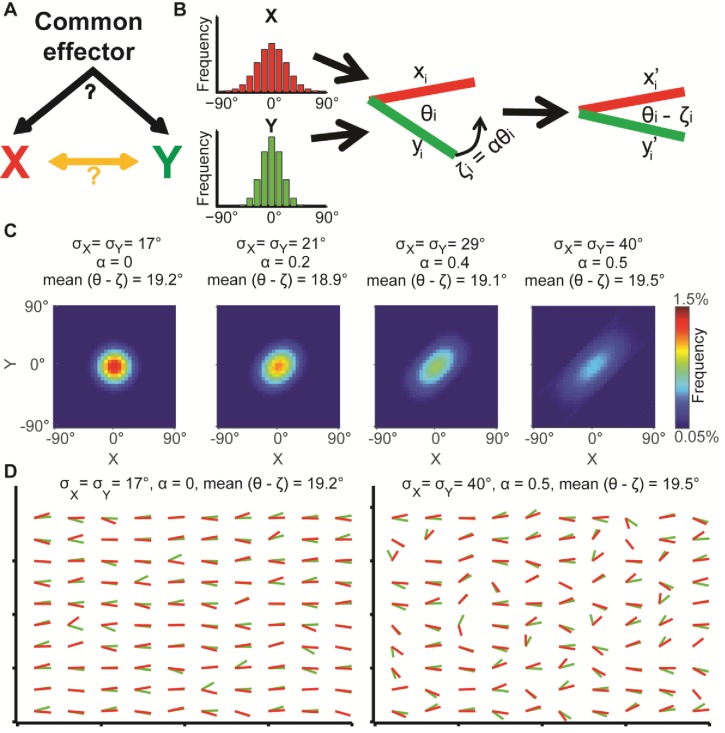
Figure 1. Illustration of global bias and local interaction using the alignment of two orientational variables.
(A) The relation between two variables X, Y can be explained from a combination of direct interactions (orange) and a common effector. (B) Simulation. Given two distributions X, Y, pairs of coupled variables are constructed by drawing sample pairs (xi,yi) and transforming them to (xi’,yi’) by a correction parameter ζi = αθi, which represents the effect of a local interaction. α is constant for each of these simulations. (C) Simulated joint distributions. X, Y truncated normal distributions with mean 0 and σX = σY. Shown are the joint distributions of 4 simulations with reduced global bias (i.e., increased standard deviation σX, σY) and increased local interaction (left-to-right). All scenarios have similar observed mean alignment of ~19°. (D) Example of 100 draws of coupled orientational variables from the two most extreme scenarios in panel C. Most orientations are aligned with the x-axis when the global bias is high and no local interaction exists (left), while the orientations are less aligned with the x-axis but maintain the mean alignment between (xi’,yi’) pairs for reduced global bias and increased local interaction (right).

