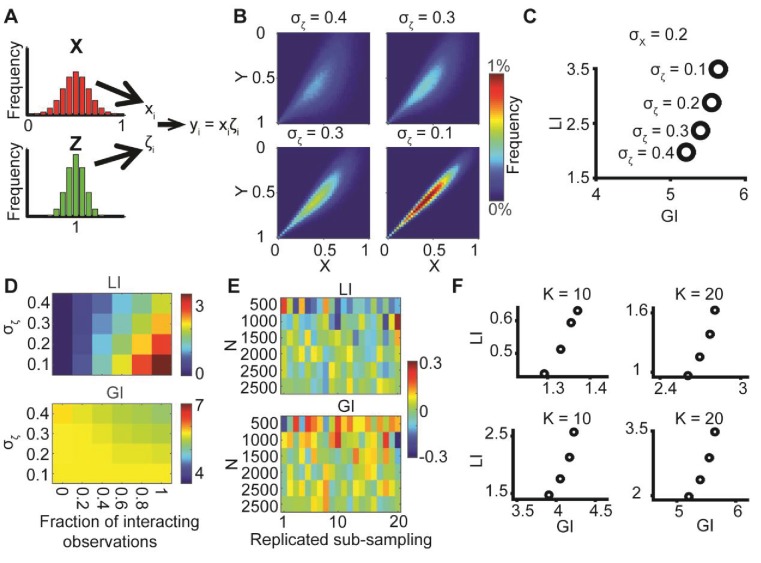
Appendix 3—figure 1. Simulating co-localization.

(A) Simulation. We use the distributions ${\displaystyle \mathrm{X}=\mathrm{N}({\mu }_x=0.5,{\sigma }_{\mathrm{x}}),\mathrm{Z}=\mathrm{N}({\mu }_{\zeta }=1,{\sigma }_{\zeta })}$, where X is truncated to [0,1]. Pairs of coupled variables are constructed by drawing sample pairs (${\displaystyle x_i,{\zeta }_i}$) and constructing ${\displaystyle y_i=x_i,{\zeta }_i}$ (Materials and methods). (B) Simulated joint distributions. Shown are the joint distributions of 4 simulations with increased global bias (i.e., decreased ${\displaystyle {\mu }_{\zeta }}$). (C) Local and global indices calculated for the examples from panel B. Smaller ${\displaystyle {\zeta }_i}$ associate with larger LI. The weaker negative association between GI and ${\displaystyle {\sigma }_{\zeta }}$ is because larger ${\displaystyle {\sigma }_{\zeta }}$induces a distribution ${\displaystyle \mathrm{Y}}$ that is more spread compared to ${\displaystyle \mathrm{X}}$ which reduces the GI. (D) Simulations of partial co-localization. A given fraction of observations for ${\displaystyle \mathrm{Y}}$ were calculated as shown in panels A–C, the rest were independently drawn from the distribution ${\displaystyle \mathrm{X}}$ implying no local interaction. Shown are LI (top) and GI (bottom) as functions of the fraction of locally interacting observations and ${\displaystyle {\sigma }_{\zeta }}$. LI associates with increased fraction of locally-interacting observations, whereas the effect is minor in GI, in accordance with panel C. (E) Deviation of LI, GI values reported in panel C as functions of the number of observations n. 20 independent sub-sampling. Lower n associates with higher variability. No other trend is observed. (F) LI and GI patterns are independent of the number of alignment histogram bins K = 10–40. Equal size of dynamic ranges was set for LI and GI plots in panels C, D and F. K, number of histogram bins was set to 40 for all panels excluding F. ${\displaystyle {\sigma }_{\mathrm{x}}}$ = 0.2 for panels B–E.

DOI: http://dx.doi.org/10.7554/eLife.22323.016