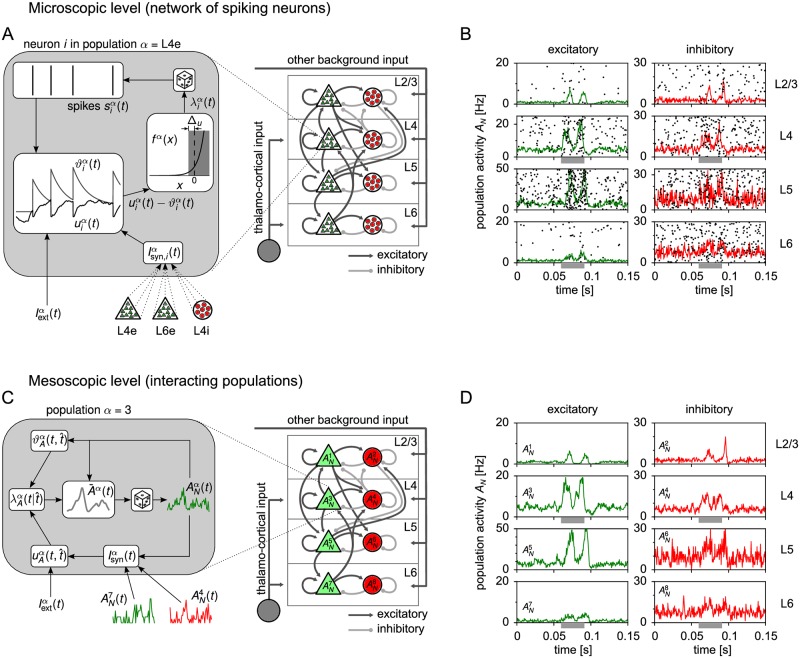
Fig 1. Illustration of population models on the microscopic and mesoscopic level.

(A) Cortical column model [5] with ∼ 80’000 neurons organized into four layers (L2/3, L4, L5, L6) each consisting of an excitatory (“e”) and an inhibitory (“i”) population. On the microscopic level, each individual neuron is described by a generalized integrate-and-fire (GIF) model with membrane potential $u_i^{\alpha }\left(t\right)$, dynamic threshold ${\vartheta }_i^{\alpha }\left(t\right)$ and conditional intensity $f^{\alpha }(u_i^{\alpha }\left(t\right)-{\vartheta }_i^{\alpha }\left(t\right))$. Inset: GIF dynamics for a specific neuron i of population L4e (α = L4e). The neuron receives spikes from neurons in L4e, L4i and L6e, which drive the membrane potential $u_i^{\alpha }\left(t\right)$. Spikes are elicited stochastically by a conditional intensity ${\lambda }_i^{\alpha }\left(t\right)=f^{\alpha }(u_i^{\alpha }\left(t\right)-{\vartheta }_i^{\alpha }\left(t\right))$ that depends on the instantaneous difference between $u_i^{\alpha }\left(t\right)$ and the dynamic threshold ${\vartheta }_i^{\alpha }\left(t\right)$. Spike feedback (voltage reset and spike-triggered threshold movement) gives rise to spike history effects like refractoriness and adaptation. (B) Spike raster plot of the first 200 neurons of each population. The panels correspond to the populations in (A). Layer 4 and 6 are stimulated by a step current during the interval (0.06s, 0.09s) mimicking thalamic input (gray bars). Solid lines show the population activities $A_N^{\alpha }\left(t\right)$ computed with temporal resolution Δt = 0.5 ms, cf. Eq (2). The activities are stochastic due to the finite population size. (C) On the mesoscopic level, the model reduces to a network of 8 populations, each represented by its population activity $A_N^{\alpha }\left(t\right)$. Inset: The mesoscopic model generates realizations of $A_N^{\alpha }\left(t\right)$ from an expected rate ${\overline{A}}^{\alpha }\left(t\right)$, which is a deterministic functional of the past population activities. (D) A corresponding simulation of the mesoscopic model yields population activities with the same temporal statistics as in (B).