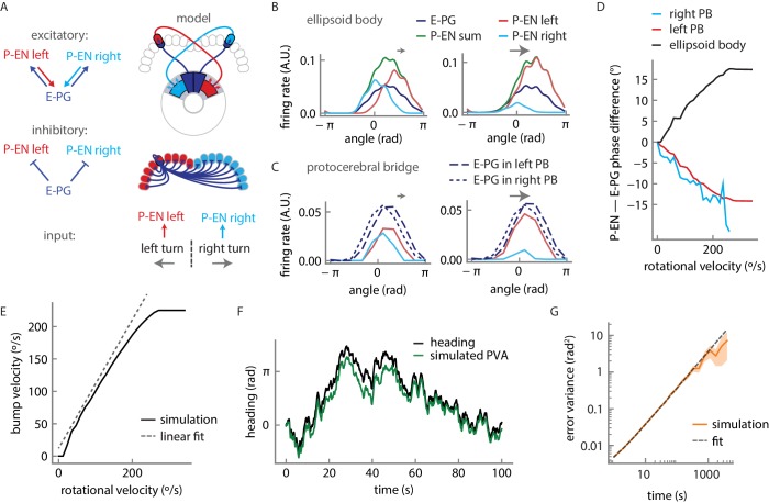
Figure 10. Firing rate model for a circuit mechanism displaying persistent localized activity and angular velocity integration.

(A) Schematic of effective excitatory (top) and inhibitory (middle) connectivity assumed in the firing rate model and external inputs to the P-EN populations (bottom). Note the anatomical shift in the ellipsoid body between E-PG and P-EN neurons relative to their protocerebral bridge connections. We assume one P-EN and three E-PG neurons per protocerebral bridge glomerulus. (B) Activity of E-PG and P-EN neurons in the ellipsoid body for counterclockwise turns at low (left, 35°/s) and high—that is, close to saturation— (right, 190°/s) angular velocities. (C) Activity of E-PG and P-EN neurons in the protocerebral bridge at low (left) and high (right) angular velocities for a snapshot in time. The velocities are the same as in B. (D) PVA difference between P-EN and E-PG bumps in the ellipsoid body (black) or protocerebral bridge (red, blue) for different angular velocities for counterclockwise turns. (E) E-PG bump velocity as a function of the fly’s rotational velocity. The bump velocity displays saturation at high velocities. A linear fit of slope one around the origin is also displayed (upward shifted for display purposes). Rotational velocities along this line will be reliably integrated. (F) Simulated PVA of the E-PG population as a function of time for a time varying rotational velocity input (see Figure 10—figure supplement 2 for a description of the input). (G) Evolution of the estimator of the error variance between the velocity input and the simulated PVA. Beyond 10 s, the statistics of the discrepancy follow a diffusion equation with a diffusion coefficient of 1.82 × 10⁻³ rad²/s (see Materials and methods for a description of the fitting procedure). The shaded area indicates the standard deviation of the estimator.

DOI: http://dx.doi.org/10.7554/eLife.23496.021

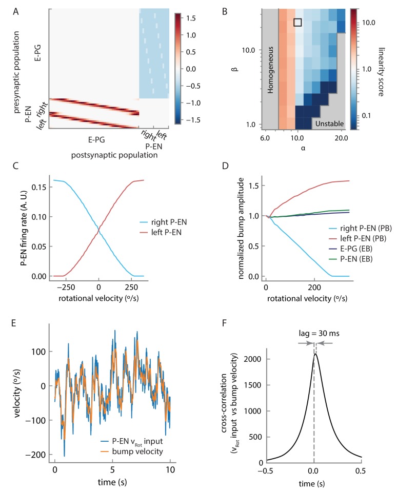
Figure 10—figure supplement 1. Model connectivity and performance.

(A) Connection matrix for the firing rate model. Note that local E-PG-to-P-EN excitation appears as a reduction in inhibition in the connectivity matrix because of strong uniform inhibition, but is converted to excitation by a constant and positive bias current in the P-EN neurons (see Materials and methods). (B) The linearity of rotational velocity integration in the model depends on the balance of local excitation and inhibition, as represented by model parameters α and β. The parameters we selected lie within the black box, that is, in a near-linear regime of velocity integration for the range of rotational velocities represented by the P-EN neuron tuning curves. Note that perfectly linear velocity integration is represented here by a linearity score of 1 (see Materials and methods). (C) Tuning curves of single, simulated P-EN neurons as a function of the velocity input. (D) Amplitude of the bumps in the ellipsoid body and the protocerebral bridge as a function of rotational velocity. (E) Velocity of the bump compared to artificially generated velocity input to P-EN neurons over a short timescale of 10 s for an artificially generated input velocity (see Figure 10—figure supplement 2 and Materials and methods). High frequencies are smoothed out, but the input is otherwise tracked well. (F) Cross-correlation of the rotational velocity input to model P-EN neurons against the velocity of the activity bump shows that the bump velocity lags the velocity input by ~30 ms. Note that this is the lag of the bump relative to the P-EN velocity input, not to the fly’s rotational velocity.

DOI: http://dx.doi.org/10.7554/eLife.23496.022

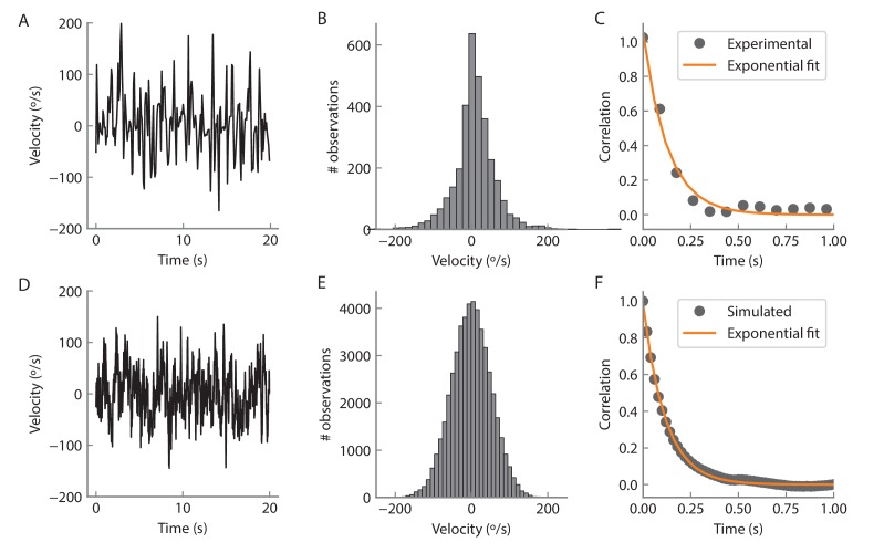
Figure 10—figure supplement 2. Angular velocity statistics.

(A) Example of an experimentally measured angular velocity track for 20 s. The velocity was downsampled to a rate of 12 Hz to match the volume imaging rate. (B) Histogram of the recorded angular velocities. The velocity was recorded over 350 s and the time points for which the angular velocity was zero were not considered for the analysis. The standard deviation of the distribution is 54°/s. (C) Time autocorrelation of the velocity tracks. The autocorrelation is well fit by an exponential with a time constant of 128 ms (orange curve). D, E, F Same as A, B, C but for a simulated track (see Materials and methods) at a rate of 50 Hz for 1000 s.

DOI: http://dx.doi.org/10.7554/eLife.23496.023