Visual extrapolation of contour geometry

Abstract

Computing the shapes of object boundaries from fragmentary image contours poses a formidable problem for the visual system. We investigated the extrapolation of contour shape by human vision. Measurements of extrapolation position and orientation were taken at six distances from the point of occlusion, thereby yielding a detailed representation of the extrapolated contours. Analyses of these measurements revealed that: (i) extrapolation curvature increases linearly with the curvature of the inducing contour, although there is individual bias in the slope; (ii) the precision with which an extrapolated contour is represented is roughly constant, in angular terms, with increasing distance from the point of occlusion; (iii) there is a substantial cost of curvature, in that the overall precision of an extrapolated contour decreases systematically with curvature; (iv) the shapes of visually extrapolated contours are characterized by a nonlinear decrease in curvature, asymptoting to zero; and (v) this decaying pattern of curvature is explained by a Bayesian model in which, with increasing distance from the point of occlusion, the prior tendency to minimize curvature gradually dominates the likelihood tendency to minimize variation in curvature.

Afundamental problem faced by the visual brain in computing object structure is the fragmentary nature of the retinal inputs. Large portions of object boundaries are often missing in the retinal images, either due to partial occlusion or because of insufficient local image contrast. Occlusion in particular poses a ubiquitous problem, given the multiplicity of objects in the world and the loss of one spatial dimension during image projection. To compute object structure from fragmented image data, the visual system must solve two related problems. It must determine (i) whether disparate image elements are in fact part of a single continuous contour (the “grouping” problem), and (ii) what shape the contour has in the missing portions (the “shape” problem).

A great deal of research has addressed the grouping problem in the contexts of partly occluded contours, illusory contours, and discretely sampled contours (1-11). This research has examined the geometric constraints that underlie the grouping of local elements into extended contours, as well as how these constraints relate to the statistics of natural images. By contrast, there has been relatively little psychophysical work on measuring the shapes of the missing portions (12-15). Because the missing portions of contours are synthesized entirely by the visual system, their detailed shapes are likely to be revealing about its underlying constraints and mechanisms.

Two constraints have been recognized in computational vision: (i) minimization of total curvature, and (ii) minimization of variation in curvature. Minimizing total curvature ∫ κ²ds (also known as “bending energy”) tends to make contours as straight as possible and leads to a class of interpolating curves known as elastica (16). Although the relevance of minimizing total curvature to the completion of extended portions of smooth contours by human vision has not been directly investigated, there is psychophysical evidence for the instantiation of a local version of this constraint in the human perception of contours. In particular, observers' ability to visually integrate local elements into extended contours deteriorates systematically with increase in curvature, defined in terms of the turning angles between successive elements (1, 3, 5, 6, 9). These results are consistent with an “association field” model of neural processing in which the pattern of connection strengths between local orientationtuned units is strongest when their preferred orientations are colinear and decreases monotonically with increasing turning angle (3, 17).† They are also consistent with the measured cooccurrence statistics of edge orientations along extended contours in natural images (9, 10).

The minimization of variation in curvature ∫ (dκ/ds)²ds, by contrast, penalizes changes in curvature rather than curvature itself. The resulting contours tend to be as close to circular as the boundary conditions will allow and lead in the context of interpolation to Euler-spiral curves (19). This minimization is consistent with the usage of edge cocircularity (or tangency to a common circle; ref. 20) to compute the strength of grouping between oriented image elements. Measurements on the statistics of natural images indeed point to a prevalence of cocircular structure in natural images (9, 21), and psychophysical work provides evidence for its role in visual contour integration (5, 22). Moreover, a recent reanalysis of physiological data suggests that the association fields of individual orientation-tuned units in the primary visual cortex may in fact be tuned to different curvatures, with the “standard” shape of the association field being a description of the population average rather than of each individual unit (23, 24).

Despite the recognition of these two constraints in computational vision, their respective contributions to contour shape completion by human vision have yet to be determined. In this article, we investigate the visual extrapolation of curved contours. Extrapolation is a critical component of the general problem of shape interpolation, given that an interpolating contour must both smoothly extrapolate each individual physically specified inducer as well as smoothly connect the two extrapolants (25, 26). More importantly, extrapolation provides a context in which the relative contributions of minimizing total curvature and minimizing variation in curvature may be readily distinguished. Minimizing total curvature exclusively results in the linear extrapolation of inducer orientation at the point of occlusion, whereas minimizing variation in curvature exclusively leads to a circular extrapolation of estimated inducer curvature. The relative contributions of the two constraints may therefore be determined by examining the pattern of curvature along visually extrapolated contours.

Experiment

We measured the perceived position and orientation of extrapolated contours at multiple distances from the point of occlusion to obtain a detailed representation of their shape. The use of smooth (rather than discretely sampled) contours and the use of occlusion (rather than a contour simply coming to an end) both serve to trigger mechanisms of visual completion, thereby generating a more vivid percept of extrapolated-contour shape.

Methods

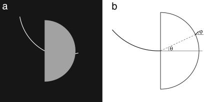
Observers viewed curved inducing contours that disappeared behind the straight edge of a half-disk occluder (Fig. 1a). An oriented-line probe protruded from behind the opposite, curved portion of the half disk (visible length = 0.17° of visual angle). Observers adjusted the position of the probe along the half-disk's circumference and its orientation, by toggling back and forth between the two adjustments, until they perceived the probe as smoothly continuing the shape of the inducing contour. Using half-disk occluders has the benefit of preserving the distance of the probe from the point of occlusion as its position is adjusted. For each inducing contour, measurements were taken with half disks of six different radii: 0.68°, 1.35°, 2.03°, 2.7°, 3.38°, and 4.06° of visual angle.

Fig. 1.

Illustration of the basic experimental stimulus. (a) Observers adjusted the position and orientation of the line probe to smoothly extrapolate the shape of the inducing contour. (b) Observer settings were measured in terms of the polar angle θ and orientation φ of the line probe relative to the inducer tangent at the point of occlusion.

Nine inducing contours were used: four circular arcs, four parabolic segments, and one linear segment. The four nonzero values of curvature (κ) at the point of occlusion were 0.059°^-1, 0.118°^-1, 0.178°^-1, and 0.237°^-1. All inducers had a visible arc length of 4.56°. They were presented at random orientations (±15°-45°), either as concave up or concave down. The inducing contours and line probe were two-pixels thick (≈2 min of arc), and antialiased to produce a smooth appearance at the resolution of 1/4 of a pixel.

Three observers, J.M.F. (O2) and two naïve, participated in eight experimental sessions each. Each session consisted of 54 trials (nine inducers × six half-disk radii), with each trial requiring combined adjustments of position and orientation. Four experimental sessions presented the inducers as concave up and four as concave down. Their order was counterbalanced.

Results

Each observer's raw data consisted of eight paired settings of angular position and orientation for each of the 54 combinations of inducing contour and occluder size. These measurements were standardized by transforming them into a single, canonical coordinate frame, one which treats the inducing contour as if it were presented horizontally at the point of occlusion and as concave up (see Fig. 1b). The standardized settings thus measure the polar angle θ and orientation φ of the adjusted probe relative to the inducer tangent at the point of occlusion. The measurements were collapsed over the concave-up and concave-down sessions because no systematic differences were obtained between them.

Observers' extrapolation of linear segments was highly accurate with no systematic bias in their positional and orientational settings (mean rms deviations from linear extrapolation: 2.45° for angular position θ, and 3.59° for orientation φ). Settings were precise, with low variability across multiple sessions (average SDs: 2.33° for angular position and 3.28° for orientation).

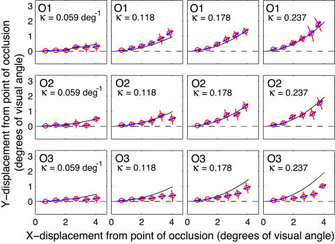
The mean settings of θ and φ for the parabolic inducers are shown, plotted in the Cartesian plane, in Fig. 2. The (curved) error bars at each radial distance denote ± 1 SD around each mean setting of angular position θ, and the error cones denote ± 1 SD around each mean setting of orientation φ.‡ Also shown on the plots are the true extensions of the parabolic curves used to generate the inducers (solid curves) and the linear extrapolants of inducer orientation at the point of occlusion (dashed lines). The corresponding plots for the circular inducers appear in Fig. 6, which is published as supporting information on the PNAS web site. We analyze these extrapolation measurements for precision, bias in shape, and the influence of inducer curvature.

Fig. 2.

Extrapolation data for the parabolic inducers. The mean settings of angular position θ and orientation φ are shown in the Cartesian plane at each of the six radial distances. Error bars for θ and error cones for φ both denote SDs. The solid curves show the extensions of the inducing parabolas, and the dashed lines show the linear extensions of the inducer tangents at the point of occlusion.

Analysis of Precision. We performed tests of heteroscedasticity to first examine the dependence of setting variability on distance from the point of occlusion (by regressing the magnitude of each data point's deviation from the mean for that radial distance against radial distance). For settings of angular position θ, only 2 of the 15 tests performed (5 curvatures × 3 observers) revealed a significant dependence of setting variance on radial distance. For settings of probe orientation φ, 4 of the 15 tests performed revealed a significant increase, and 1 test revealed a significant decrease. Thus, on the whole, there is little evidence for a systematic increase in setting variability as a function of radial distance. This result implies that the precision with which an extrapolated contour is represented is roughly constant, in angular terms, as a function of distance from the point of occlusion. A constant standard deviation in the angular position implies that SDs in Cartesian position exhibit a scalar increase with distance from the point of occlusion. These results are thus consistent with the Weber law-like dependence found in previous studies on the extrapolation of linear motion and of the direction of a static line segment (27, 28). The current results extend these previous findings to the case of curved contours.

To examine the influence of inducer curvature on precision, the SDs were collapsed over all six radial distances [i.e., 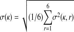], thereby yielding overall measures of precision with which angular position and orientation are represented along an extrapolated contour. All six tests performed (two angular measurements for three observers) revealed significant heteroscedasticity, in particular, a significant increase in setting variance as a function of inducer curvature. Thus, there is a significant “cost of curvature” (13), in that the overall precision of an extrapolated contour decreases systematically with increasing curvature of the inducing contour. For angular position, the average SDs across the three observers increased from 2.33° for linear inducers to 5.73° for the highest-curvature inducers. For orientation, they increased from 3.28° to 9.56° (see Fig. 7, which is published as supporting information on the PNAS web site).

Analysis of Bias. To model the curvature of extrapolated contours, we computed for each inducer the best-fitting (maximum-likelihood) parabolic curve to the combined extrapolation data.

We defined the likelihood model as follows:

[1]

This model defines, for each curvature value κ (here, of a parabola at its vertex), the probability of obtaining a given extrapolation dataset , where r indexes the six radial distances, and i indexes the eight repeated measurements. θ_p(κ, r) and φ_p(κ, r) are the ideal values based on the extension of the parabola used to define the inducer. Based on the analysis of precision, the SDs σ_θ and σ_φ were taken to be independent of radial distance and estimated from the extrapolation data for each inducing contour.§

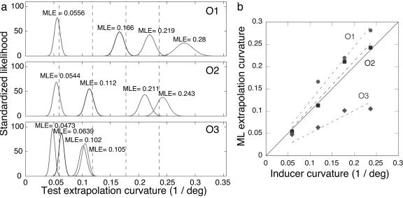
Fig. 3a shows the standardized likelihood functions (i.e., normalized to have unit mass) computed for the observers' extrapolations of the four parabolic inducers.¶ Fig. 3b plots the maximum-likelihood estimates of extrapolation curvature against inducer curvature. For all three observers, the curvatures of the extrapolated contours depend linearly on inducer curvature (R values for a scalar-increase model: 0.985, 0.983, and 0.845), but the slope of this dependence varies (1.22, 1.06, and 0.55). Relative to the true curvature values used to generate the parabolic inducers, observers O1 and O2 exhibit a slight overestimation of curvature (by 22% and 6%, respectively), whereas O3 exhibits a substantial underestimation (by 45%).

Fig. 3.

Standardized likelihood functions and maximum-likelihood estimates for the extrapolation data with parabolic inducers. (a) Standardized likelihood functions on extrapolation curvature corresponding to the four inducer curvatures at the point of occulsion. The dashed lines mark the inducer curvatures at the point of occlusion. (b) Maximum-likelihood estimates of extrapolation curvature plotted as a function of inducer curvature.

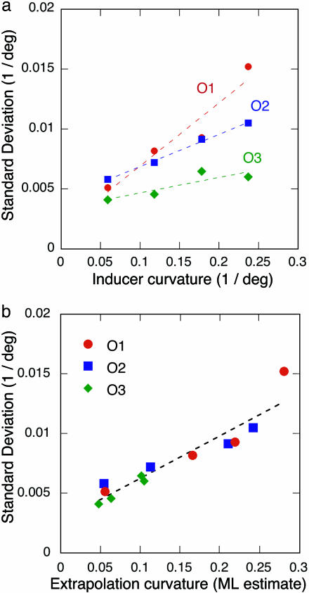
Fig. 4a shows the standard deviations of the standardized likelihood functions plotted as a function of inducer curvature. For each observer, these increase linearly as a function of inducer curvature (R values for a linear model: 0.958, 0.998, and 0.872). Increase in the spread of the standardized likelihood function signifies an increase in uncertainty in observers' estimate of the curvature of the extrapolated contour (see ¶). We observed previously that the variance in observers' local settings of angular position θ and orientation φ increased systematically with inducer curvature. The current analysis demonstrates this cost of curvature in a more direct way, i.e., by exhibiting greater uncertainty in observers' estimates of extrapolation curvature for inducers with higher curvature.

Fig. 4.

SDs of the standardized likelihood functions. (a) SDs plotted as a function of inducer curvature. (b) SDs plotted as a function of estimated extrapolation curvature. Despite the individual bias in extrapolation curvature, a single linear equation captures the dependence of these SD on extrapolation curvature for all three observers (O1-O3).

When the same SDs are plotted against estimated extrapolation curvature, rather than inducer curvature (see Fig. 4b), the data points from all observers fall along a single line. Thus, despite the individual differences in the curvatures of the extrapolated contours, a single linear equation models the dependence of the SD on extrapolation curvature for all three observers (y = 0.0355x + 0.0027, R = 0.942). The more highly curved an observer's extrapolated contour is, the weaker the overall precision with which it is represented.

Shape Models

Circular and Parabolic Models. In characterizing the geometry of the observed extrapolated contours, we compare the fits of various shape models. We begin by considering a circular model M_c and a parabolic model M_p, each having a single parameter κ (the curvature of the circle, and the curvature of the parabola at its vertex). Given that these models are not nested, classical Neyman-Pearson techniques for model selection are not applicable. However, Bayesian techniques have been developed, based on the work of Jeffreys (31), to compare nonnested models. These techniques rely on the notion of the Bayes factor, which is the ratio of (marginal) likelihoods p(D|M_p)/p(D|M_c) under the two models (32).∥

The Bayes factor essentially captures how one's prior belief concerning the two models [as expressed in the prior odds, ], is transformed into the posterior belief [as expressed in the posterior odds, ], as a result of the measurements 𝒟. In the absence of any prior preference for either model [], the Bayes Factor simply gives the posterior odds. Each (marginal) probability in the Bayes Factor is computed by conditionalizing with respect to the parameter κ of the model and integrating

[2]

where the second equality follows under minimally informative prior distributions on κ under both models, i.e., locally uniform in the region of interest, and zero elsewhere. Bayes factor values for the extrapolation data were thus computed by taking the ratios, under the two models, of the areas under their likelihood curves.

For both parabolic and circular inducers, these Bayes factors were consistently >1 (in all 24 cases: three observers × four curvatures × two inducer shapes; see Table 1, which is published as supporting information on the PNAS web site). Thus, the parabolic model provides a better fit than the circular model, not only to the extrapolations of the parabolic inducers but also to those of the circular inducers. In considering why this might be so, note that an important difference between the two models is that, starting from its vertex (the “initial” point for our parabolic model), the curvature of the parabola decreases monotonically with arc length, whereas the curvature of the circle is constant. A natural hypothesis, therefore, is that visually extrapolated contours have the property that their curvature decreases systematically with distance from the point of occlusion. The parabolic model performs better because it is able to model this decreasing-curvature trend, whereas the circular model is not.

Spiral Models. We test the above “decreasing-curvature hypothesis” by fitting spiral models to the extrapolation data. Because spirals are characterized by a monotonic variation in curvature, the best-fitting parameters of a spiral model can naturally indicate whether there is a systematic tendency for the curvature of extrapolated contours to decrease.

The simplest form of monotonic variation in curvature, namely a linear increase or decrease, defines an Euler spiral (also known as the Cornu spiral or the clothoid). We define an Euler spiral model with two parameters: the initial curvature κ and the constant slope in curvature γ. The curvature profile of this spiral is thus given by κ(s) = κ + γs, where s is arc length. γ > 0 corresponds to a linear increase in curvature, γ < 0 to a linear decrease, and γ = 0 to the degenerate case of a circular arc.

To estimate the best-fitting Euler spirals to the extrapolation data, we use a likelihood model with the same functional form as before (Eq. 1). The ideal settings of angular position θ_e(κ, γ, r) and orientation φ_e(κ, γ, r) at each radial distance are now derived from the general form of the Euler spiral (19). Fig. 8, which is published as supporting information on the PNAS web site, shows the contour plots of the likelihood surfaces for the fits of the Euler spiral model. In 23 of 24 cases, the maximum-likelihood estimates for the rate-of-change-of-curvature term γ are negative. By comparing the fits of the Euler spiral to the degenerate case of the circular model (by using nested-model hypothesis tests; see Table 2, which is published as supporting information on the PNAS web site), we found that 18 of these 23 negative values were significantly different from 0 (the positive value was not).

The fits of the Euler spiral model thus provide strong evidence for the decreasing-curvature hypothesis. However, the Euler spiral cannot be taken as a general model of extrapolated contour shape. Because its decrease in curvature is linear, the Euler spiral eventually reverses its sign of curvature, clearly an undesirable property. A more reasonable pattern of behavior is one in which the curvature converges asymptotically on 0. A well-known spiral that has this property is the logarithmic spiral (also known as the equiangular spiral, or the growth spiral). In its most general form, its curvature profile is defined by κ(s) = 1/(bs + a), where s is arc length. Based on this curvature profile, we derive a general Cartesian form for the log spiral (see Supporting Derivation, which is published as supporting information on the PNAS web site) and define a two-parameter model in terms of the spiral's initial curvature κ = 1/a and its initial rate of change curvature γ = -b/a².

To compare the fits of the logarithmic-spiral model and Euler-spiral model (two nonnested models with two parameters each), we again use Bayes Factors. Assuming no prior preference for either model and minimally informative prior distributions on their parameters κ and γ, the Bayes factor for the log-spiral model M_ls against the Euler-spiral model M_es is given by the ratio of the integrated likelihoods ∫ ∫ p(D|κ, γ) dκ dγ under the two models. These marginal likelihoods were approximated by numerical integration of the volumes under the likelihood surfaces of the two models. The resulting values of the Bayes factor ratios for the extrapolation data with both parabolic and circular inducers were consistently >1 (Table 3, which is published as supporting information on the PNAS web site), indicating that the logarithmic spiral provides a superior fit to the extrapolation data than the Euler spiral model.

Bayesian Contour Extrapolation

We outline a Bayesian model that captures the decaying-curvature behavior of visually extrapolated contours. Based on the association-field model of connectivity between orientation-tuned units in the primary visual cortex and extensive behavioral data on the visual system's preference for colinearity of local elements in contour integration (3, 5, 6, 9), we take the prior distribution on contour curvature to be a Gaussian centered on zero, that is p(κ_e) ∼ N(0, σ_pr) for some σ_pr. This prior simply entails that, in the absence of any image information, the visual system's default preference is for a contour to go straight.

The likelihood, which reflects the information derived from the image data, is taken to be based on a process that estimates the curvature of a contour segment and then simply extends the contour while maintaining this curvature, i.e., in a cocircular fashion. Again, there is a great deal of evidence for cocircularity from the statistics of natural images (9, 21), psychophysical performance in contour integration (5, 22), and a recent reanalysis of physiological data (24). Thus, the mean of the likelihood function is taken to be the estimated curvature of the inducing contour at the point of occlusion, . A critical assumption of the model is that the spread of the likelihood increases monotonically with distance from the point of occlusion. In other words, the continuation of estimated inducer curvature is subject to systematically greater noise, with increasing distance from the point of occlusion. We assume a Weber-like dependence, namely, a linear increase in SD with radial distance: σ_lik(r) = σ_lik(0) + mr, where σ_lik(0) is the SD when gap size is zero (infinitesimally thin occluder). Thus, ).

Given the assumption that the prior distribution and likelihood are both Gaussians, there exist well known analytic formulas for the posterior (30). In particular, the posterior is also a Gaussian with the mean given by

[3]

Substituting the appropriate values of means and SDs, we obtain the following expression for the (maximum a posteriori) curvature estimate of the extrapolated contour at each radial distance r

[4]

Setting r = 0, we obtain ). Thus, the “initial” curvature of the extrapolated contour is a function of the relative sizes of and . Under the natural assumption that the continuation of estimated inducer curvature is subject to very little noise at or near the point of occlusion, we have σ_lik(0) ≪ σ_pr and, therefore, ; that is, the extrapolation curvature near the point of occlusion essentially equals the estimated inducer curvature. On the other hand, if one considers the possibility that σ_lik (0) is approximately equal to σ_pr, then the initial extrapolation curvature would have one-half of the magnitude of the estimated inducer curvature.

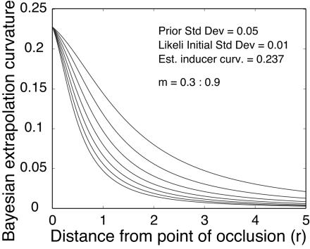
From Eq. 4, it also follows that with increasing distance from the point of occlusion (i.e., as r → ∞), the curvature of the extrapolated contour decreases asymptotically to zero (i.e., ) at a rate that is modulated by the slope term m (Fig. 9, which is published as supporting information on the PNAS web site). This decay is consistent with the pattern of curvature observed along visually extrapolated contours.

Fig. 5 shows the decay of curvature of the Bayesian extrapolated contour as a function of radial distance for different values of m. The plots in this figure correspond to the situation where the spread of the likelihood near the point of occlusion, σ_lik(0), is substantially smaller than the spread of the prior distribution, σ_pr. Consistent with the above analysis, the curvature of the extrapolated contour near the point of occlusion essentially equals the estimated inducer curvature.

Fig. 5.

Plots showing the variation of curvature along Bayesian extrapolated contours as a function of distance from the point of occlusion. The curvature decreases asymptotically to zero at a rate modulated by the slope term m. This decay is consistent with the pattern of curvature observed along visually extrapolated contours.

Thus, under simple and natural assumptions concerning the prior and likelihood distributions, the Bayesian model captures the pattern of decaying curvature seen in observers' extrapolated contours. Moreover, by manipulating the relative magnitudes of the standard deviation of the prior distribution and the initial SD of the likelihood, it can capture the individual variability seen in the overall curvature of observers' extrapolated contours.

Conclusions

Dependence of Extrapolation Shape on Curvature. The visual system systematically takes into account the curvature of inducing contours when extrapolating their shapes. Each observer exhibited a linear increase in extrapolation curvature with inducer curvature, although there was individual bias in the slope. Most current models of contour completion take into account only the positions and orientations of the inducing contours. The current results show that a successful model must take into account their curvatures as well.

Constant Precision in Angular Terms. The variability in positional and orientational settings is roughly constant, in angular terms, at different points along an extrapolated contour. A constant SD in angular position implies linearly increasing SDs in Cartesian position as a function of distance from the point of occlusion. This result extends previous findings on the extrapolation of linear direction to the case of curved contours.

Cost of Curvature. The precision with which an extrapolated contour is represented becomes systematically weaker with increasing curvature. This weakening of precision correlates more strongly with extrapolation curvature than with inducer curvature. Indeed, despite the individual bias in the curvature of the extrapolated contours, all observers exhibited essentially the same linear dependence on extrapolation curvature (see Fig. 4).

Extrapolation Shape Characterized by Decaying Curvature. The shapes of extrapolated contours were consistently captured better by a parabolic model than a circular model, regardless of whether the inducing contours were parabolic or circular. This result motivated the decreasing-curvature hypothesis, which was then directly tested and supported by the fits of an Euler spiral model. Fits of a logarithmic spiral model further clarified that a nonlinear decrease in curvature, asymptoting to zero, better describes the shapes of visually extrapolated contours than a linear decrease.

Bayesian Model Captures Curvature Decay. A Bayesian model clarifies how the two constraints of minimizing curvature (or tendency toward colinearity) and minimizing variation in curvature (or tendency toward cocircularity) interact to produce the observed pattern of decaying curvature along visually extrapolated contours. The tendency toward colinearity is embodied in the prior distribution, whereas the tendency toward cocircularity is embodied in the likelihood. The shapes of visually extrapolated contours derive from the relative strengths of these two constraints at different distances from the point of occlusion. Near the point of occlusion, the likelihood dominates the prior, with the result that the extrapolated contour is maximally curved. With increasing distance from the point of occlusion, the influence of the likelihood weakens (as a result of an increase in its spread) so that the prior gradually comes to dominate the likelihood. This shift in relative weights leads to a systematic decay in the curvature of the extrapolated contour.

The current study also raises intriguing questions concerning how well human observers will perform in extrapolating natural contours that contain structure at multiple scales and how the application of the current model may be extended to include such cases. These and other related questions await systematic investigation.

References

- 1.Uttal, W. R. (1973) Vision Res. 13, 2155-2163. [DOI] [PubMed] [Google Scholar]
- 2.Kellman, P. J. & Shipley, T. F. (1991) Cognit. Psychol. 23, 141-221. [DOI] [PubMed] [Google Scholar]
- 3.Field, D., Hayes, A. & Hess, R. (1993) Vision Res. 33, 173-193. [DOI] [PubMed] [Google Scholar]
- 4.Ringach, D. L. & Shapley, R. (1996) Vision Res. 36, 3037-3050. [DOI] [PubMed] [Google Scholar]
- 5.Feldman, J. (1997) Vision Res. 37, 2835-2848. [DOI] [PubMed] [Google Scholar]
- 6.Pettet, M. W. (1999) Vision Res. 39, 551-557. [DOI] [PubMed] [Google Scholar]
- 7.Singh, M. & Hoffman, D. D. (1999) Percept. Psychophys. 61, 943-951. [DOI] [PubMed] [Google Scholar]
- 8.Feldman, J. (2001) Percept. Psychophys. 63, 1171-1182. [DOI] [PubMed] [Google Scholar]
- 9.Geisler, W. S., Perry, J., Super, B. & Gallogly, D. (2001) Vision Res. 41, 711-724. [DOI] [PubMed] [Google Scholar]
- 10.Elder, J. H. & Goldberg, R. M. (2002) J. Vision 2, 324-353. [DOI] [PubMed] [Google Scholar]
- 11.Anderson, B. L., Singh, M. & Fleming, R. (2002) Cognit. Psych. 44, 148-190. [DOI] [PubMed] [Google Scholar]
- 12.Anderson, B. L. & Barth, H. C. (1999) Neuron 24, 433-441. [DOI] [PubMed] [Google Scholar]
- 13.Warren, P. A., Maloney, L. T. & Landy, M. S. (2002) Vision Res. 42, 2431-2446. [DOI] [PubMed] [Google Scholar]
- 14.Singh, M. (2004) Psych. Sci. 15, 454-459. [DOI] [PubMed] [Google Scholar]
- 15.Guttman, S. E. & Kellman, P. J. (2004) Vision Res. 44, 1799-1815. [DOI] [PubMed] [Google Scholar]
- 16.Mumford, D. (1994) in Algebraic Geometry and Its Applications, ed. Bajaj, C. L. (Springer-Verlag, New York), pp. 491-506.
- 17.Grossberg, S. & Mingolla, E. (1985) Psych. Rev. 92, 173-211. [PubMed] [Google Scholar]
- 18.Feldman, J. & Singh, M. (2005) Psych. Rev. 112, 243-252. [DOI] [PubMed] [Google Scholar]
- 19.Kimia, B. B., Frankel, I. & Popescu, A. (2003) Int. J. Comp. Vision 54, 157-180. [Google Scholar]
- 20.Parent, P. & Zucker, S. W. (1989) IEEE Trans. Pattern Anal. Mach. Intell. 11, 823-839. [Google Scholar]
- 21.Sigman, M., Cecchi, G. A., Gilbert, C. D. & Magnasco, M. O. (2001) Proc. Natl. Acad. Sci. USA 98, 1935-1949. [DOI] [PMC free article] [PubMed] [Google Scholar]
- 22.Pizlo, Z., Salach-Goyska, M. & Rosenfeld, A. (1997) Vision Res. 37, 1217-1241. [DOI] [PubMed] [Google Scholar]
- 23.Bosking, W., Zhang, Y. & Fitzpatrick, D. (1997) J. Neurosci. 17, 2112-2127. [DOI] [PMC free article] [PubMed] [Google Scholar]
- 24.Ben-Shahar, O. & Zucker, S. W. (2004) Neural Comp. 16, 445-476. [DOI] [PubMed] [Google Scholar]
- 25.Ullman. S. (1976) Biol. Cybern. 25, 1-6. [Google Scholar]
- 26.Fantoni, C. & Gerbino, W. (2003) J. Vision 3, 281-303. [DOI] [PubMed] [Google Scholar]
- 27.Salomon, A. D. (1947) Am. J. Psych. 60, 68-88. [PubMed] [Google Scholar]
- 28.Pavel, M., Cunningham, H. & Stone, V. (1992) Vision Res. 32, 2177-2186. [DOI] [PubMed] [Google Scholar]
- 29.Mardia, K. V. (1972) Statistics of Directional Data (Academic, London).
- 30.Box, G. E. P. & Tiao, G. C. (1992) Bayesian Inference in Statistical Analysis (Wiley, New York).
- 31.Jeffreys, H. (1961) Theory of Probability (Oxford Univ. Press, Oxford), 3rd Ed.
- 32.Kass, R. E. & Raftery, A. E. (1995) J. Amer. Stat. Assoc. 90, 773-795. [Google Scholar]
Associated Data
This section collects any data citations, data availability statements, or supplementary materials included in this article.