Figure 4.

Modeling Melanopsin’s Contribution to Spatial Vision

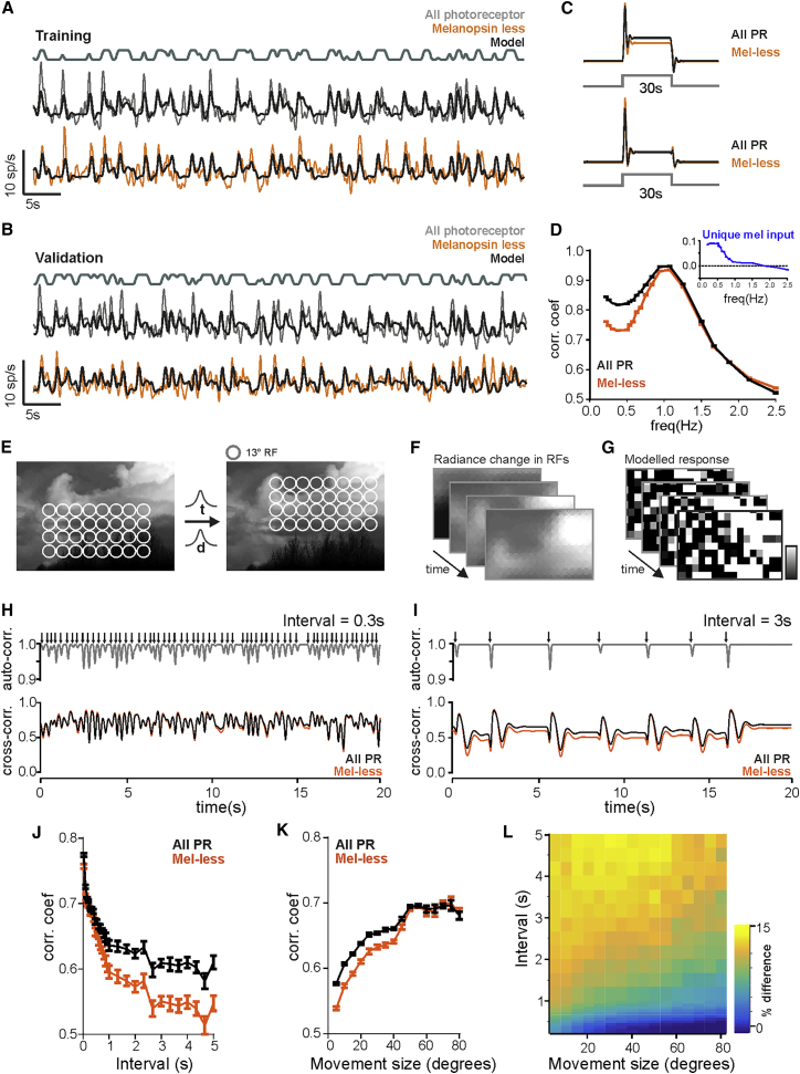
(A) Responses to the binary modulation stimulus rendered in “all-photoreceptor” or “melanopsin-less” stimuli (mean responses of 11 MR units [from 56 units recorded in five animals] for a 60-s epoch shown with gray and orange lines, respectively) were fitted using an autoregressive exogenous (ARX) model (thick black line). Above gray line shows model input (smoothed stimulus).

(B) Models were validated on a separate response epoch to the binary modulation stimulus (mean responses for a 60-s epoch shown with gray and orange lines, for “all-photoreceptor” and “melanopsin-less,” respectively; thick black line shows model prediction). Above gray line shows model input (smoothed stimulus).

(C) Model-predicted responses to a 30 light step rendered in “all-photoreceptor” (black) and “melanopsin-less” (orange) for MR units (top) and non-MR units (bottom). Stimulus presentation depicted with gray lines.

(D) Mean ± SEM correlation between stimulus and modeled responses generated for “all-photoreceptor” (black) and “melanopsin-less” (orange) conditions for a range of binary modulation stimuli spanning different frequency ranges (summarized in Figure S3F; repeated for 25 modeled neurons). Correlation coefficients were significantly different at frequencies <1 Hz. Inset: unique melanopsin input (“all-photoreceptor” – “melanopsin-less” response).

(E–G) Cartoon depicting the process of modeling MR unit responses over space and time. Natural images were tiled with an array of MR unit RFs (E) (13° diameter). The array of MR RFs was then moved across the natural image with a range of intervals (t) and distances (d). The image was filtered through the overlapping array of modeled RFs (F). The correlation coefficient between stimulus and the modeled responses (G) of an array of neurons tiling the natural image was then calculated for each frame in a 30-s epoch.

(H and I) Images were moved across an array of RFs (mean distance = 30°) for mean intervals of 0.3 s (H) and 3 s (I). Arrows depict movement events over a 20-s epoch. Top: spatial autocorrelation between frames (low correlation occurring following image movement). Bottom: spatial cross-correlation between stimulus and modeled responses for each frame over time (“all-photoreceptor” and “melanopsin-less” linear filters depicted with black and orange lines respectively). Note elevated cross-correlation in “all-photoreceptor” model for periods of high auto-correlation in (I).

(J) Mean ± SEM correlation coefficient for a range of intervals (mean interval between movement of 0.03–5 s), for a fixed movement size (mean ± SD 10° ± 3°), for “all-photoreceptor” and “melanopsin-less” models (black and orange lines, respectively). Significant differences in correlation were found at intervals >0.4 s).

(K) Mean ± SEM correlation coefficient for a range of movement sizes (mean amplitudes of 5°–80°), for a fixed inter-stimulus interval (mean ± SD 1 ± 0.3 s), for “all-photoreceptor” and “melanopsin-less” models (black and orange lines, respectively). Significant differences in correlation were found at movement sizes <45°).

(L) Heatmap showing % difference in correlation values generated for “all-photoreceptor” and “melanopsin-less” responses modeled across a range of intervals (0.03–5 s) and amplitudes (5°–80°).

See also Figure S3.