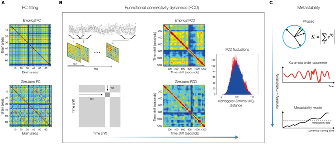
Figure 1.

Methods for measuring fit between simulated and empirical data. (A) The fitting of the FC is measured by the Pearson correlation coefficient between corresponding elements of the upper triangular part of the matrices. (B) For comparing the FCD statistics, we collected the upper triangular elements of the matrices (over all participants or sessions) and compared the simulated and empirical distribution by means of the Kolmogorov-Smirnov distance between them. The Kolmogorov–Smirnov distance quantifies the maximal difference between the cumulative distribution functions of the two samples. (C) We measure the metastability as the standard deviation of the Kuramoto order parameter across time. The Kuramoto order parameter measures the global level of synchronization of the n oscillating signals. Under complete independence, the n phases are uniformly distributed and thus R is nearly zero, whereas R = 1 if all phases are equal (full synchronization). For calculating the metastability of the empirical and simulated BOLD signals, we first band-pass filtered within the narrowband 0.04–0.07 Hz and computed the instantaneous phase φ_k(t) of each narrowband signal k using the Hilbert transform. The Hilbert transform yields the associated analytical signals. The analytic signal represents a narrowband signal, s(t), in the time domain as a rotating vector with an instantaneous phase, φ(t), and an instantaneous amplitude, A(t). Bottom panel visualizes a single example scenario (of many possible others) where the model system’s metastability increases as a function of G. We also indicate the metastability measured in empirical data. Part of figure B is based on the work of Allen and colleagues⁴⁴.