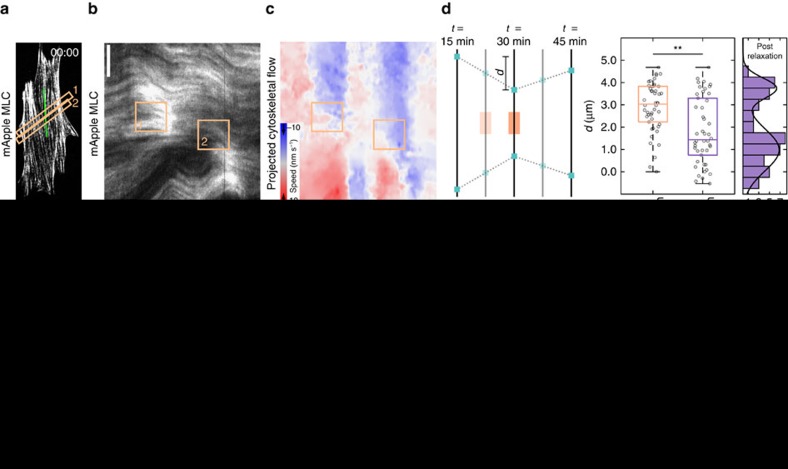
Figure 4. Stress fibres behave elastically.
(a) Image showing a cell labelled with mApple-MLC. The activation regions are indicated by the orange boxes. (b) A kymograph drawn along the stress fibre (green line in panel a). During activation periods, myosin flows towards the activation regions. (c) A kymograph created from the same region as panel b using the flow maps determined previously. Flow was projected onto the stress fibre and colour coded to indicate speed and direction. This flow map illustrates that, during relaxation periods, myosin flow reverses direction away from the activation periods. (d) A quantification of displacement of stress fibres during contraction and relaxation. Puncta ∼5 μm from the activation zone were tracked and measured following 15 min of activation and again following 15 min of relaxation (n=41 from 4 cells). Puncta translated about 3 μm from their original position and relaxed to ∼1 μm from their original position elastically. The relaxation response could be further broken into two groups, one with a strong reversal (∼80% of their original position) and one with a weak reversal (∼25% of their original position). (e) A cell transfected with mApple-α-actinin. The activation area is indicated by the orange box. (f) A kymograph drawn along the direction indicated in panel e, overlain with tracks of the individual α-actinin puncta during activation. (g) The velocity of individual puncta along the stress fibre is measured from the slope of the tracks and plotted against the distance from the activation region. Adjacent puncta all move at approximately the same speed. Sudden changes in velocity (blue arrowhead) correlate with what appear to be site of mechanical failure along the stress fibre and the appearance of new puncta. The black line represents the stress fibre from panel f, while the grey lines are other stress fibres from the same cell. (h) A representative kymograph is fit to both the 1D continuum and 2D discrete models. Both models are able to recapitulate the flow patterns seen experimentally. Scale bars are 10 μm in panels a,e. Horizontal scale bars are 15 min and vertical scale bars are 5 μm in panels b,f,h. **P<0.01, two-sample Student's t-test.

