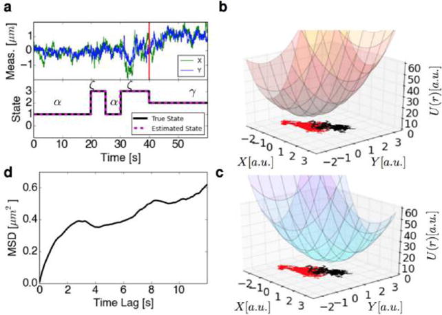
Figure 34.

Nonparametric Bayesian analysis is helpful to SPT trajectory analysis. (a) Position trajectory of a 2D simulation illustrating nonlinear time dependent kinetics; the bottom portion of the plot displays the true state label as well as the number of states (and label) inferred by the HDP-SLDS algorithm.⁶⁸ The vertical red line denotes the point at which the potential abruptly changes; potential before and after this change are plotted in rightmost panels. (b) The potential energy surface governing the particle dynamics before an abrupt state change in the position of the potential energy’s global minimum location at t = 40 s. The x and y coordinates of the measured position are plotted; the portion of the trajectory governed by the potential plotted in this panel is colored in red. (c) Potential energy surface of trajectory after an abrupt state change in the position corresponding to the potential energy’s minimum location at t = 40 s. The x and y coordinates of the measured position are plotted; the portion of the trajectory subject to the potential plotted in this panel is colored in black. (d) The MSD curve of the simulated trajectory exhibiting transitions between three types of diffusive motion; the MSD was computed using all measurements shown in the top left panel. See text for additional discussion. The data set for this simulation was created by a simple Gillespie algorithm while the labels and number of states were found via a simple MATLAB implementation of the HDP-SLDS algorithm.⁶⁸ Standard MATLAB functions were used to calculate the MSD.