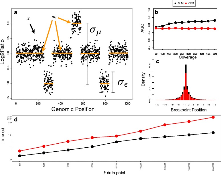
Fig. 1.

Performance comparison between SLM and CBS algorithms on simulated data. Panel a shows how genomic profiles are modeled by SLM. Black dots are the observations x _i, orange segments are the unobserved mean levels m _i and vertical black bars represent the ranges of ${\sigma }_m^2$ and ${\sigma }_{\epsilon }^2$. Panel b reports the area under the receiver operating characteristic curve (AUC) as a function of sequencing coverage for SML and CBS. Panels c summarizes the performance of SLM and CBS algorithms in the detection of the correct breakpoint position, while panel d reports the computational speed of the two methods in segmenting genomic profiles made of different number of data points (analyses were performed on a 2.5 GHz Intel Core i5 with 8 Gb of RAM). Black dots represent SLM, while red ones CBS. On the x axis of panel c is reported the distance between the predicted and the correct breakpoint position, while on the y axis is reported the fraction of breakpoints predicted at a given distance from the correct position