IMPROVING PARAMETER INFERENCE FROM FRAP DATA

Abstract

Fluorescence recovery after photobleaching (FRAP) is used to obtain quantitative information about molecular diffusion and binding kinetics at both cell and tissue levels of organization. FRAP models have been proposed to estimate the diffusion coefficients and binding kinetic parameters of species for a variety of biological systems and experimental settings. However it is not clear what the connection among the diverse parameter estimates from different models of the same system is, whether the assumptions made in the model are appropriate, and what the qualities of the estimates are. Here we propose a new approach to investigate the discrepancies between parameters estimated from different models. We use a theoretical model to simulate the dynamics of a FRAP experiment and generate the data that is used in various recovery models to estimate the corresponding parameters. By postulating a recovery model identical to the theoretical model, we first establish that the appropriate choice of observation time can significantly improve the quality of estimates, especially when the diffusion and binding kinetics are not well balanced, in a sense made precise later. Secondly, we find that changing the balance between diffusion and binding kinetics by changing the size of the bleaching region, which gives rise to different FRAP curves, provides a priori knowledge of diffusion and binding kinetics, which is important for model formulation. We also show that the use of the spatial information in FRAP provides better parameter estimation. By varying the recovery model from a fixed theoretical model, we show that a simplified recovery model can adequately describe the FRAP process in some circumstances, and establish the relationship between parameters in the theoretical model and those in the recovery model. We then analyze an example in which the data is generated with a model of intermediate complexity and the parameters are estimated using models of greater or less complexity, and show how sensitivity analysis can be used to improve FRAP model formulation. Lastly, we show how sophisticated global sensitivity analysis can be used to detect over-fitting with a model being too complex.

1 Introduction

Pattern formation in developmental biology is currently an active interdisciplinary area between biologists and physical scientists because the interaction of experimentation and modeling has produced significant new insights into a number of model systems. At the cell and tissue level pattern formation involves several distinct elements: a signal of some sort, signal relay either via direct communication between cells or via a longer-range transport process such as diffusion, and mechanisms for detecting that signal and acting on it. Turing (1952) called the signals morphogens, and his seminal paper and the later paper by Wolpert (1969) provided a framework within which to formulate hypotheses about pattern formation and differential gene expression. The availability of experimental data for Bicoid (Driever and Nüsslein-Volhard 1988; Driever and Nüsslein-Volhard 1988) and other morphogens (Lander 2007; Reeves et al. 2006) has led to a shift from predominantly phenomenological models of pattern formation to mechanism-based models, the purposes of which are not only to explain the existing observations within a mechanistic framework, but also to serve as tools for discovery by experimentalists. Mathematical models for Drosophila oogenesis, Bicoid patterning, BMP-mediated patterning, planar cell polarity, EGF patterning, and segment polarity have all led to experiments that may not have been carried out otherwise, and contributed greatly to our understanding of those systems (Shvartsman et al. 2002; Amonlirdviman et al. 2005; Yakoby et al. 2005; Goentoro et al. 2006; Umulis et al. 2006; Perkins et al. 2006; Serpe et al. 2008).

An important and often difficult step in testing models against experimental observations is the determination of model parameters from limited data when details of the mechanistic steps involved are not known. In particular, it is difficult to determine whether the postulated model is too simple or too complex for the given data. Our objective here is to show how using different combinations of spatial and temporal data can improve parameter estimation in a postulated model, and how post-processing with sensitivity analysis can be used to address the complexity issue. An example described later that arose from studies of the Drosophila wing disc (Kicheva et al. 2007; Zhou et al. 2012) illustrates this in detail, which is also the motivation of our study in FRAP.

1.1 Background on FRAP and an outline of the paper

FRAP is a widely-used technique for quantitative measurement of molecular dynamics. The literature on FRAP analysis is large and can only be touched upon here, but a recent review is given in (Beaudouin et al. 2013). Some background information relevant to our analysis is given in the Appendix, but the essential facts needed are as follows. In a FRAP experiment, the fluorescence-tagged molecules in a region of interest (ROI) are first photobleached, and then the recovery of fluorescence within the ROI due to transport from the surrounding region is recorded (Braeckmans et al. 2003). By fitting the recovery data to a mathematical model, parameters that measure transport due to diffusion, binding and chemical reactions can be estimated. The data obtained is usually averaged over the ROI and presented as a recovery curve such as shown in Figure 1. The notation used in the figure is as follows. Let b = Ω_ROI/Ω denote the ratio of the area of the ROI to the area of the entire domain. Let a be the ratio of the remaining fluorescent intensity after bleaching to the fluorescent intensity before bleaching, assuming that bleaching is homogeneous and instantaneous, and let c be the fraction of fluorescent molecules which are immobile on the time scale of the experiment. The loss of fluorescence due to bleaching reflected in a recovery curve is b(1 − a), and the immobile fraction outside the ROI is c(1 − b).

Figure 1.

A typical recovery curve for a FRAP experiment. After subtraction of the background fluorescence and correction of the observed photobleaching, a FRAP recovery curve is normalized by the fluorescent intensity before bleaching. See text for explanation of the symbols.

The FRAP recovery curve is usually normalized as

$${\mathrm{F}}_{\mathit{norm}}(\mathrm{t})=\frac{\mathrm{F}(\mathrm{t})-\mathrm{F}({\mathrm{T}}_0)}{(1-\mathrm{b})(1-\mathrm{c})+\text{ab}},$$

where in F is the fluorescence intensity and t ≥ T₀ + T₁ (Hinow et al. 2006; Braeckmans et al. 2007). Later we assume that bleaching is complete, i.e., a = 0, and that no immobile fraction exists, i.e., c = 0.

The parameter estimation step consists in fitting this data with a ‘suitable’ model, but since the recovery portion typically can be fit with a sum of time-dependent exponential terms (Mai et al. 2011), this leaves wide latitude as to what underlying processes are to be included, and once that is fixed, what meaning can be ascribed to those parameters. Traditionally FRAP experiments were used for cellular or sub-cellular level processes that occur on short time scales, and by fitting parameters such as diffusion coefficients and binding rates to the data, properties of cell- or sub-cellular-level processes could be inferred. More recently FRAP has been used for tissue-level studies that occur on a long time scale, where the results may be influenced by the interactions of production, transport, decay and other processes (Kicheva et al. 2007; Zhou et al. 2012; Müller et al. 2012; Müller et al. 2013), and a major issue in the use of FRAP in this context is what model should be used as the basis for parameter estimation. This latitude can lead to wide discrepancies in the estimated parameters, since one recovery model may omit a process included in another. Even if the recovery models are identical, the parameter estimates may vary widely due to differences in the assumptions about the parameters, as will be described in an example later. Therefore, to the extent possible, a careful assessment of whether and how the transport and reaction processes couple should be made before a FRAP model is formulated, because otherwise the results may bear little relationship to the actual processes that determine the recovery curve.

To demonstrate the effect of different model assumptions and different ways of utilizing the data from a FRAP experiment, we avoid the above difficulties of unknown mechanisms and other factors by generating data computationally for a known model with known parameters and then testing our recovery of parameters from the data. By using a recovery model identical to the theoretical model, we show that the choice of observation time can significantly affect the estimates. We also show that changing the bleaching region to rebalance the diffusion and binding processes can significantly improve the estimates. By varying the recovery model from the theoretical model, we investigate whether the simplified recovery model can, in some circumstances, appropriately describe the FRAP process, the relationship between parameters in the theoretical model and those in the recovery model, and under what conditions some processes can be neglected in the recovery model. Lastly, we introduce sensitivity analysis as a technique to better understand FRAP data and to improve FRAP model formulation.

In the following section we begin with a simple example in which the parameters of a complex model can be related to parameters in a simplified description. We then develop and solve the evolution equation from which the parameters are estimated in a standard experiment, and we describe the computational setup and the analysis of the data. We provide a detailed analysis of simplified diffusion-reaction models of FRAP, and use these to show how the neglect of processes in FRAP lead to erroneous estimation. For simplicity we assume throughout that diffusion is the only spatial transport process involved (internalization of receptor-ligand complexes is allowed, as discussed later). We provide the solution for models with influx (or production) and decay. We further restrict attention to geometrically one-dimensional systems, but the method can easily be generalized to 2D or 3D, and can be used to study more complicated questions in FRAP, for example, when binding is nonlinear. We believe it advances our understanding of the limitations of the existing FRAP experiments and models, helps to reconcile the parameter estimates in biological systems, and will direct the improvement of the FRAP technique.

2 The mathematical framework for parameter estimation and model testing

We begin the mathematical description of FRAP with a simplified geometric description of a wing disc for the purpose of (i) emphasizing the assumptions implicit, but rarely discussed, in many FRAP analyses, and (ii) showing that coefficients extracted for a simple description may reflect more complicated processes than the usual interpretation of parameters would suggest. A general formulation of the linear reaction-diffusion systems that govern FRAP analysis is given in the Appendix A.1. As shown in Figure 2, the geometry of the disc is complex, and morphogen transport in the disc may involve several different mechanisms that are discussed later. This gives rise to challenges of model determination, parameter estimation and interpretation when using FRAP. However, a careful analysis with detailed model testing can provide significant insights into the underlying mechanism.

Figure 2.

Patterning of epithelial cells in the Drosophila wing imaginal disc. The morphogen Dpp patterns the Anterior/Posterior compartments of the Drosophila wing imaginal disc in (A) top view showing the pouch and (B) slice (along dotted line in (A)) showing the geometry of the columnar cells. (C–D) Dpp establishes a non-uniform distribution to pattern the anterior/posterior axis by transport and reaction. Numerous processes may contribute to formation of the Dpp distribution including diffusion around columnar cells (C) or transcytosis through columnar cells (D). Dpp secreted in the basolateral space cannot enter the lumen and vice versa due to the presence of septate junctions (SJ) in (D). From (Othmer et al. 2009) with permission.

For simplicity we consider a thin fluid layer (Figure 3), equivalent to the lumen in the wing disc, and admit diffusion, binding to surface-bound receptor, and internalization and re-expression of receptors to emphasize assumptions implicit in most analyses. We assume that the surface reactions involve only binding to a receptor and decay of the receptor-ligand complex, and to simplify the analysis, we suppose that whenever a receptor-ligand complex is internalized it is replaced by a bare receptor (Umulis et al. 2006). We measure receptor and receptor-ligand concentrations in molecules or moles per unit area, and we assume that the steps by which an occupied receptor is internalized and a free receptor is recycled to the surface reach a steady state rapidly compared with other processes, which implies that the total amount of receptor is constant at every point on the surface z = 0, i.e., $R+\overline{\mathit{RC}}=R_T$ where R_T is a constant. We further assume that the turnover is sufficiently rapid to balance the influx at the boundary so that a steady state of the full system exists.

Figure 3.

The geometry of a thin fluid layer over receptors embedded in a surface. Modified from (Umulis et al. 2008).

The surface z = 0 can be regarded as the outer cell boundary of a sheet of cells covered by a thin layer of fluid, as in a simplified description of the Drosophila wing disc. The lengths in the x, y and z directions are L_x, L_y, and L_z, respectively, and we let C be the concentration of a morphogen in the fluid and R the concentration of receptor on the surface z = 0. Suppose there is a fixed influx of C on the boundary x = 0 that is uniform in the y and z directions, and zero flux on the remaining faces except z = 0. Then the governing equations can be written as follows.

$$\begin{array}{lll}\frac{\partial C}{\partial t}=D\mathrm{\Delta }C\hfill & \text{in}\hfill & \mathrm{\Omega }\hfill \end{array}$$ (2.1)

$$\begin{array}{lll}\frac{\partial R}{\partial t}=-k^{+}RC+(k^{-}+k_e)\overline{\mathit{RC}}\hfill & \text{on}\hfill & z=0\hfill \end{array}$$ (2.2)

$$\begin{array}{lll}\frac{\partial \overline{\mathit{RC}}}{\partial t}=k^{+}RC-(k^{-}+k_e)\overline{\mathit{RC}}\hfill & \text{on}\hfill & z=0\hfill \end{array}$$ (2.3)

$$\begin{array}{lll}-D\frac{\partial C}{\partial z}=-k^{+}RC+k^{-}\overline{\mathit{RC}}\hfill & \text{on}\hfill & z=0\hfill \end{array}$$ (2.4)

$$\begin{array}{lll}-D\frac{\partial C}{\partial x}=j\hfill & \text{on}\hfill & x=0\hfill \end{array}$$ (2.5)

$$\begin{array}{lll}D\frac{\partial C}{\partial x}=0\hfill & \text{on}\hfill & x=L_x\hfill \end{array}$$ (2.6)

where k⁺ and k⁻ are the binding and dissociation rates between ligand and receptor, and k_e is the decay rate of the receptor-ligand complex.

This system can be simplified by defining the dimensionless variables u = C/C₀, v = R/R_T, $w=\overline{\mathit{RC}}/R_T$, the scaled coordinates ξ = x/L_x, η = y/L_y and ζ = z/L_Z, and the dimensionaless time τ = t/T. The system then becomes

$$\begin{array}{lll}\frac{\partial u}{\partial \tau }=\frac{\mathit{DT}}{L_x^2}\left(\frac{{\partial }^{2}u}{\partial {\xi }^2}+\frac{L_x^2}{L_y^2}\frac{{\partial }^{2}u}{\partial {\eta }^2}+\frac{L_x^2}{L_z^2}\frac{{\partial }^{2}u}{\partial {\zeta }^2}\right)\hfill & \text{in}\hfill & \mathrm{\Omega }\hfill \end{array}$$ (2.7)

$$\begin{array}{lll}\frac{\partial v}{\partial \tau }=-T{k}^{+}{C}_0{R}_{T}uv+T(k^{-}+k_e)(1-v)\hfill & \text{at}\hfill & \zeta =0\hfill \end{array}$$ (2.8)

$$\begin{array}{lll}-\left(\frac{D{C}_0}{L_z}\right)\frac{\partial u}{\partial \zeta }=-k^{+}{R}_T{C}_{0}uv+k^{-}(1-v)\hfill & \text{at}\hfill & \zeta =0\hfill \end{array}$$ (2.9)

$$\begin{array}{lll}-\frac{\partial u}{\partial \xi }=\frac{j{L}_x}{D{C}_0}\hfill & \text{at}\hfill & \xi =0\hfill \end{array}$$ (2.10)

$$\begin{array}{lll}\frac{\partial u}{\partial \xi }=0\hfill & \text{at}\hfill & \xi =1\hfill \end{array}$$ (2.11)

In view of the boundary conditions the solution must be constant in the η direction at steady state, and we assume this for the transient problem as well. Furthermore, since the fluid layer is thin L_z ≪ L_x, L_y, and the equations can be averaged over ζ. In this case the equations reduce to

$$\begin{array}{lll}\frac{\partial \overline{u}}{\partial \tau }=\left(\frac{\mathit{DT}}{L_x^2}\right)\frac{{\partial }^2\overline{u}}{\partial {\xi }^2}-T{k}^{+}{R}_T\overline{u}\overline{v}+\left(\frac{T{k}^{-}{R}_T}{C_0}\right)(1-\overline{v})\hfill & \text{in}\hfill & \mathrm{\Omega }\hfill \\ \frac{\partial v}{\partial \tau }=-T{k}^{+}{C}_0\overline{u}\overline{v}+T(k^{-}+k_e)(1-\overline{v})\hfill & \text{at}\hfill & \zeta =0\hfill \\ -\frac{\partial \overline{u}}{\partial \xi }=\frac{j{L}_x}{D{C}_0}\hfill & \text{at}\hfill & \xi =0\hfill \\ \frac{\partial \overline{u}}{\partial \xi }=0\hfill & \text{at}\hfill & \xi =1\hfill \end{array}$$ (2.12)

where $\overline{u}$ and $\overline{v}$ are the averages over ζ. At steady state the system reduces to

$$\begin{array}{lll}\frac{d^{2}u}{d{\xi }^2}={\gamma }^2\frac{u}{K+u}\hfill & \text{in}\hfill & \mathrm{\Omega }\hfill \\ -\frac{\mathit{du}}{d\xi }=J\hfill & \text{at}\hfill & \xi =0\hfill \\ \frac{\mathit{du}}{d\xi }=0\hfill & \text{at}\hfill & \xi =1\hfill \end{array}$$ (2.13)

where u now stands for the average over ζ, and

$$\begin{array}{lll}K=\frac{k^{-}+k_e}{k^{+}{C}_0}\hfill & {\gamma }^2=\frac{k_e{R}_T{L}_x^2}{D{C}_0{L}_z}\hfill & J=\frac{j{L}_x}{D{C}_0}\hfill \end{array}.$$

If u ≪ K, which means that the dimensionless concentration is far from the saturation level, this reduces to

$$\begin{array}{lll}\frac{d^{2}u}{d{\xi }^2}={\delta }^{2}u\hfill & \text{in}\hfill & \mathrm{\Omega }\hfill \\ -\frac{\mathit{du}}{d\xi }=J\hfill & \text{at}\hfill & \xi =0\hfill \\ \frac{\mathit{du}}{d\xi }=0\hfill & \text{at}\hfill & \xi =1\hfill \end{array}$$ (2.14)

where

$${\delta }^2=\frac{k_e{k}^{+}}{k^{-}+k_e}\frac{R_T{L}_x^2}{D{L}_z}\equiv k_s\frac{R_T{L}_x^2}{D{L}_z}.$$

The dimensionless solution u is

$$u(\xi )=\frac{J}{\delta }\left[\frac{e^{\delta (1-\xi )}+e^{-\delta (1-\xi )}}{e^{\delta }-e^{-\delta }}\right]=\frac{J}{\delta }\varphi (\xi ).$$ (2.15)

The stationary distribution is characterized by two dimensionless parameters: δ and J. The first is the square root of the ratio of a diffusion time scale τ_D and a kinetic time scale τ_K ≡ k⁻¹, and the second is the ratio of the input flux j to a characteristic velocity defined by the diffusion constant and the decay rate. The former enters in the shape function ϕ via the exponential terms and determines how rapidly the morphogen concentration decays in space: the larger δ the more rapidly the solution decays from the value at the source. Thus reducing the kinetic scale by reducing the half-life of the morphogen, or increasing the diffusion time scale by decreasing the diffusion constant, leads to sharper, more rapidly-decreasing spatial profiles. It should also be noted that the second term in both the numerator and denominator of (2.15) arises from the finite length of the domain, and can only be neglected if δ ≫ 1.

While it is sometimes assumed that δ also controls the approach to the steady state, the following shows that this is not correct. To illustrate this as simply as possible, consider the transient version of (2.14), which reads

$$\begin{array}{ll}\frac{\partial c}{\partial \tau }=\frac{{\partial }^{2}c}{\partial {\xi }^2}-{\delta }^{2}c\hfill & \xi \in (0,1)\hfill \\ -\frac{\partial c}{\partial \xi }=J\hfill & \xi =0\hfill \\ \frac{\partial c}{\partial \xi }=0\hfill & \xi =1\hfill \\ c(\xi ,0)=0.\hfill & \xi \in (0,1)\hfill \end{array}$$ (2.16)

The approach to steady state is governed by the evolution of the difference w ≡ u−u^s, where u^s is the steady state solution (2.15). This satisfies (2.16) with J = 0 and w(ξ, 0) = −u^s(ξ), and the solution is

$$w(\xi ,\tau )={\displaystyle \sum _{n=1}^{\infty }{a}_n{e}^{-{\mathrm{\lambda }}_n\tau }\cos n\pi \xi },$$ (2.17)

wherein the constants a_n are determined by the steady-state solution. The exponential decay rates λ_n are given by

$${\mathrm{\lambda }}_n={\left(n\pi \right)}^2+{\delta }^{2}n=1,2,\dots$$ (2.18)

and the smallest of these, λ₁, defines the relaxation time of the slowest decaying mode cos(πξ) in the transient solution. The reciprocal of this is a dimensionless relaxation time, and converting it to dimensional form one finds that the relaxation time to the steady state is given by

$$T_R\equiv \frac{1}{\frac{D{\pi }^2}{L^2}+k}=\frac{1}{\frac{{\pi }^2}{{\tau }_D}+\frac{1}{{\tau }_K}}.$$ (2.19)

This shows that either morphogen diffusion or morphogen decay can dominate the relaxation process, and their effect is additive. The relaxation time increases with a decrease in D or an increase in L, while the effect of the morphogen decay is independent of the space scale. In the context of the Drosophila wing disc the half life of the morphogen Dpp has been estimated as 45 min, and the diffusion coefficient is estimated to be 0.1 μm²/sec (Kicheva et al. 2007). For a disc of 50μm the diffusion factor in the denominator of (2.19) is 0.0204, while the second factor is 0.022, which leads to a relaxation time of about 24 minutes. On the other hand, if the diffusion coefficient is 20 μm²/sec (Zhou et al. 2012) the relaxation time is reduced to ∼ 0.25 minutes. While the disparity in this example arises from the different choices of the diffusion coefficient, in general the relaxation to a steady state following a perturbation can be used experimentally to gain additional information about the underlying processes.

In case the smaller value of D obtains, diffusion and decay are balanced on the scale of the wing disc, but in other systems the conclusion may be quite different. In the context of Drosophila embryonic development, the half-life of the transcription factor Bicoid has been estimated to range from ∼ 8 mins (Spirov et al. 2009) to less than ∼ 30 mins (Grimm et al. 2010), and if we use 20 mins as an intermediate estimate, k = 0.05 min⁻¹. Estimates of the diffusion coefficient range upward from 0.3 μm²/sec (Grimm et al. 2010), and thus for the lowest D and an embryo length of L = 500μm, the relaxation time of the slowest decaying mode is ∼20 mins, and is determined almost solely by the degradation rate.

Several assumptions are noteworthy. Firstly, u represents the average concentration over the thickness of the fluid layer due to the averaging over ζ. This is an appropriate description for most FRAP experiments, in which averaging over the ROI precedes the parameter estimation, but it must be noted that receptor concentrations have to be defined appropriately, and that the interpretation of binding constants reflects this. Secondly, though the steady-state problem with binding and internalization leads to the simple problem at (2.14), the parameter δ comprises several parameters that describe binding and internalization, and thus interpreting this as a simple decay constant is generally not valid.

2.1 The computational FRAP setup

To investigate different approaches to the analysis of FRAP data, we use a computational model to generate the FRAP data, which facilitates evaluation of the effect of experimental parameters such as the size of the ROI and the time of observation. In our simulations the FRAP data is generated by using the dimensionless form of equations as (A.5) described except that real time is used, i.e., without scaling.

The geometry of the tissue can be described as an approximately rectangular compartment, and when the bleaching is done in a stripe as in Figure 4 ((Kicheva et al. 2007; Zhou et al. 2012)), the concentration of fluorescent molecules varies primarily in one direction (x above), variations are negligible in the y direction under no-flux boundary conditions in that direction, and are typically recorded as the maximum projection in the z direction. Under these conditions the data analysis can be reduced to a one dimensional problem. Accordingly, in this paper the mathematical formulation and all simulations are done only in 1D. However, the conclusions and numerical procedure in our 1D system can be applied and easily extended to 2D and 3D systems.

Figure 4.

Left: A region of the wing disc that is scanned (from (Kicheva et al. 2007) with permission). Green indicates GFP-labelled Dpp, the white box is the ROI, and the scale bar is 10μm, Right: Adapted from (Hinow et al. 2006). (top) The computational approximation of the disc as an ellipse and the rectangular ROI, (bottom) the initial data along a one-dimensional cross-section of the region.

FRAP recovery data is the spatial average of the sum of free and bound fluorescence in the observation region, which may be smaller that the ROI, so suppose that u₁ represents the free molecule and other species u_i, i > 1 are bound species. Then the fluorescence intensity as a function of time τ is described as

$$\overline{u_i(\tau )}=\frac{1}{l_R-l_L}{\displaystyle {\int }_{l_L}^{l_R}{u}_i(\xi ,\tau )d\xi }\mathit{frap}(\tau )={\displaystyle \sum _{i=1}^m\overline{u_i(\tau )}}$$ (2.20)

where $1>l_R=\frac{L_R}{L}>l_L=\frac{L_L}{L}>0$. Here L is the overall size of the system¹, and L_L and L_R define the observation region. The problem of parameter estimation can be considered as an inverse problem or optimization process, and the algorithm underlying our method is shown in Figure 5, and the mathematical details are given in the next section. In practice, the number of terms (M) that are retained in the eigenfunction expansion is determined by setting a threshold for changes and increasing the number of terms until the parameter estimates do not change within the threshold.

Figure 5.

The computational algorithm used throughout the paper.

Another issue that arises in parameter estimation concerns the initial condition for the recovery equation (Mueller et al. 2008). It is well known that during the bleaching phase bleached and unbleached molecules diffuse in and out of the ROI, and this results in a transition region with various levels of photobleaching between the bleached and unbleached region. The size of the intermediate region depends on the molecular diffusivity, size of the bleaching region and the bleaching time. It may have substantial effects on the estimation of molecular motility and binding kinetics. In this paper, we assume that the bleaching process is instantaneous and use piece-wise constant data as shown in Figure 4 as the initial data for simulations unless specified otherwise.

3 Theoretical models for FRAP data generation

We examine two classes of theoretical models – which are summarized in Table 1 – one in which the system is closed and a second one in which there is a specified flux at the boundary. We briefly present the governing equations and some basic results in this section to make it easier for the reader to compare the models. In the following section we use the models in computational studies to show how parameter estimates depend on the model used and how they can be improved with different protocols.

Table 1.

Summary of the models for the following analysis and simulations. Numbers in parentheses refer to the subsections in which the corresponding model is introduced (3.x.x) and the computational results are given (4.x.x).

	FRAP models for closed systems	FRAP models with boundary fluxes
1-component model	Model B1 (4.2.1)	Model B2 (4.2.3)
	$\frac{\partial u_1}{\partial \tau }=D_1{\nabla }^2{u}_1$	$\frac{\partial u_1}{\partial \tau }=D_1{\nabla }^2{u}_1-k^d{u}_1$
	$-D_1\frac{\partial u_1}{\partial \xi }{|}_{\xi =0}=0$	$-D_1\frac{\partial u_1}{\partial \xi }{|}_{\xi =0}=J$
	$-D_1\frac{\partial u_1}{\partial \xi }{|}_{\xi =1}=0$	$-D_1\frac{\partial u_1}{\partial \xi }{|}_{\xi =1}=0$
2-component model	Model 1 (3.1.1, 4.1.1–4.1.5, 4.2.1, 4.2.2)	Model 3 (3.2.1, 4.1.6, 4.2.3)
	$\frac{\partial u_1}{\partial \tau }=D_1{\nabla }^2{u}_1-k^{+}{u}_1+k^{-}{u}_2$	$\frac{\partial u_1}{\partial \tau }=D_1{\nabla }^2{u}_1-k^{+}{u}_1+k^{-}{u}_2$
	$\frac{\partial u_2}{\partial \tau }=k^{+}{u}_1-k^{-}{u}_2$	$\frac{\partial u_2}{\partial \tau }=k^{+}{u}_1-k^{-}{u}_2-k^d{u}_2$
	$-D_1\frac{\partial u_1}{\partial \xi }{|}_{\xi =0}=0$	$-D_1\frac{\partial u_1}{\partial \xi }{|}_{\xi =0}=J$
	$-D_1\frac{\partial u_1}{\partial \xi }{|}_{\xi =1}=0$	$-D_1\frac{\partial u_1}{\partial \xi }{|}_{\xi =1}=0$
3-component model	Model 2 (3.1.2, 4.1.6, 4.2.2)	Model 4 (3.2.2, 4.1.6, 4.2.3)
	$\frac{\partial u_1}{\partial \tau }=D_1{\nabla }^2{u}_1-k_1^{+}{u}_1+k_1^{-}{u}_2-k_2^{+}{u}_1+k_2^{-}{u}_3$	$\frac{\partial u_1}{\partial \tau }=D_1{\nabla }^2{u}_1-k^{+}{u}_1+k^{-}{u}_2$
	$\frac{\partial u_2}{\partial \tau }=k_1^{+}{u}_1-k_1^{-}{u}_2$	$\frac{\partial u_2}{\partial \tau }=k^{+}{u}_1-k^{-}{u}_2-k^i{u}_2$
	$\frac{\partial u_3}{\partial \tau }=k_2^{+}{u}_1-k_2^{-}{u}_3$	$\frac{\partial u_3}{\partial \tau }=k^i{u}_2-k^d{u}_3$
	$-D_1\frac{\partial u_1}{\partial \xi }{|}_{\xi =0}=0$	$-D_1\frac{\partial u_1}{\partial \xi }{|}_{\xi =0}=J$
	$-D_1\frac{\partial u_1}{\partial \xi }{|}_{\xi =1}=0$	$-D_1\frac{\partial u_1}{\partial \xi }{|}_{\xi =1}=0$

3.1 FRAP models for closed systems

3.1.1 Model 1: one mobile species and one type of binding site

In the simplest model there is one diffusible fluorescent species U₁ that can bind to an immobile receptor R to produce the complex U₂ (Sprague et al. 2004), according to the reaction $U_1+R\underset{k^{-}}{\overset{k^{+}}{\rightleftharpoons }}{U}_2$. As stated earlier and shown in Appendix A.4, the recovery process can be modeled as a linear process and this leads to a solution of the form (A.9), where u₁, u₂ denote the concentration of unbound and bound fluorescent molecules, resp.,², and

$$K=\left(\begin{array}{cc}-k^{+}& k^{-}\\ k^{+}& -k^{-}\end{array}\right)D=\left(\begin{array}{cc}{D}_1& 0\\ 0& 0\end{array}\right)$$

and ϕ_n = cos(nπξ), and ${\alpha }_n^2={\left(n\pi \right)}^2$. Both K and D are singular, the former due to the conservation condition³.

We denote by I₀ the total initial concentrations and show in Appendix A.4 that the initial fractions are

$$\begin{array}{ccc}{u}_{10}=\frac{I_0}{1+K_d^{-1}}& \text{and}& u_{20}=\frac{I_0}{1+K_d}\end{array}.$$

where K_d ≡ k⁻/k⁺ is the dissociation constant. In addition, $k^{+}=k^{+}([R_T]-u_2^{ts})$ and k⁻ = k⁻, where R_T, $u_2^{ts}$ denote the total binding sites and the total concentration of bound molecules, respectively. Note that these two quantities are constant throughout the FRAP experiment. The initial conditions are

$${\left(\begin{array}{c}{u}_1\\ u_2\end{array}\right)}_{\tau =0}={\displaystyle \sum _{n=0}^{\infty }\left(\begin{array}{c}{y}_{1n}\\ y_{2n}\end{array}\right)\mathit{cos}(n\pi \xi )}=\left(\begin{array}{c}{u}_{10}\\ u_{20}\end{array}\right)$$ (3.1)

where u₁₀, u₂₀ are the initial concentrations of unbound and bound fluorescent molecules after photobleaching, respectively. The coefficients y_1n, y_2n are given by

$$\begin{array}{cc}{y}_{10}={\displaystyle {\int }_0^1{u}_{10}(x)dx}& y_{1n}=2{\displaystyle {\int }_0^1{u}_{10}(x)\mathit{cos}(nx)dx}\end{array}$$

and

$$\begin{array}{cc}{y}_{20}={\displaystyle {\int }_0^1{u}_{20}(x)dx}& y_{2n}=2{\displaystyle {\int }_0^1{u}_{20}(x)\mathit{cos}(nx)dx}\end{array}.$$

The average fluorescence intensities of bound and unbound molecules across the ROI during the recovery phase are given by

$$\begin{array}{l}\left(\begin{array}{c}{\overline{u}}_1\\ {\overline{u}}_2\end{array}\right)=\frac{1}{{\delta }^{-}}{\displaystyle {\int }_{l_L}^{l_R}\left(\begin{array}{c}{u}_1(\tau ,\xi )\\ u_2(\tau ,\xi )\end{array}\right)d\xi }\\ =e^{K\tau }{y}_0+\frac{1}{\pi {\delta }^{-}}{\displaystyle \sum _{n=1}^{\infty }\frac{1}{n}\left[\mathit{sin}(n\pi l_R)-\mathit{sin}(n\pi l_L)\right]e^{[K-D{\left(n\pi \right)}^2]\tau }{y}_n}\end{array}$$ (3.2)

$$=e^{K\tau }{y}_0+\frac{1}{\pi {\delta }^{-}}{\displaystyle \sum _{n=1}^{\infty }\frac{1}{n}\left[\mathit{sin}\frac{(n\pi {\delta }^{-})}{2}\mathit{cos}\frac{(n\pi {\delta }^{+})}{2}\right]e^{[K-D{\left(n\pi \right)}^2]\tau }{y}_n}$$ (3.3)

where y_n = (y_1n, y₂)^T, and δ^± = l_R ±l_L. Finally, the average fluorescence intensity in time, i.e., the FRAP data, is given by

$$\mathit{frap}(\tau )=\overline{u_1}(\tau )+\overline{u_2}(\tau ).$$ (3.4)

The parameter space for this two-component diffusion-binding model can be divided into several regimes that reflect different balances between the component processes. There are three different characteristic time scales in the system: the diffusion time τ_D = (δ⁻)²/D where δ⁻ is the width of the bleaching region, the binding time τ_b = 1/k⁺, and the dissociation time τ_dis = 1/k⁻. In the initial stages of recovery the primary effect of diffusion is from a small region adjacent to the bleached region into the bleached region, and therefore we use a characteristic diffusion time based on the width of the ROI. When binding is weak, i.e., τ_dis/τ_b ≪ 1, and the diffusion is not much faster than binding, i.e., above τ_D/τ_b ≪ 1, the recovery process can be described by pure diffusion, in which case the parameters are located in the pure diffusion regime of Figure 6. When binding is tighter, i.e., τ_dis/τ_b ≫ 1, and much faster than diffusion, i.e., τ_D/τ_b ≫ 1, the recovery process can be approximated as a diffusion process but with an effective diffusion coefficient $D_{\mathit{eff}}=D/(1+K_d^{-1})$, and the parameters are located in the effective diffusion regime. When the binding is tighter, i.e., right τ_dis/τ_b ≥ 1, and diffusion is much faster than binding τ_D/τ_b ≪ 1, the recovery time is determined by the reaction process when the parameters are located in reaction-dominant regime. Outside the three special regimes, the remainder of the parameter space is called diffusion-reaction regime. For the upcoming discussion, it is worth noticing that the diffusion characteristic time can be manipulated by the spatial scale of the bleaching region, which could lead to a shift of the location of parameters from one regime to another.

Figure 6.

Different regimes in the parameter space for a diffusion binding model (Adapted from (Sprague et al. 2004)).

3.1.2 Model 2: one mobile species and multiple types of binding sites

To illustrate the different scales that arise with multiple binding sites, consider two sites, for which K and D can be obtained from Appendix (A.2). When the binding steps are much faster than diffusion this is the case treated earlier, and the effective diffusion coefficient given at (A.23) takes the form D_eff = D₁/(1 + K₂ + K₃), where $K_2=k_1^{+}/k_1^{-}$, $K_3=k_2^{+}/k_2^{-}$.

Suppose however that binding to the second type reaches a quasi-steady state rapidly compared to binding to the first and to diffusion. Then local equilibrium gives rise to u₃ = K₃u₁, and by adding the governing equations, we have

$$\frac{\partial }{\partial \tau }(u_1+u_3)=D{\nabla }^2{u}_1-k_1^{+}{u}_1+k_1^{-}{u}_2$$

By dividing the equations for u₁ and u₂ by 1 + K₃ one can reduce to a model with a single binding site, which reads

$$\frac{\partial u_1}{\partial \tau }=D_{\mathit{rd}}{\nabla }^2{u}_1-k^{+}{u}_1+k^{-}{u}_2^{\prime }$$ (3.5)

$$\frac{\partial }{\partial \tau }(u_2^{\prime })=k^{+}{u}_1-k^{-}{u}_2^{\prime }$$ (3.6)

where

$$u_2^{\prime }=\frac{u_2}{1+K_3},D_{\mathit{rd}}=\frac{D_1}{1+K_3},k^{+}=\frac{k_{21}}{1+K_3},\text{and}{k}^{-}=\frac{k_{12}}{1+K_3}.$$

These parameters are what are obtained in the parameter estimation when the two-site model is reduced to a model with a single binding site as above, and illustrate again that the estimated parameters may be complex functions of the more fundamental parameters.

3.2 FRAP models with boundary fluxes

3.2.1 Model 3: Influx, diffusion, binding and decay

The parameters measured from different time and space scales may reflect different integration of biological processes such as production, internalization and decay in addition to diffusion and binding discussed above. In biological systems at tissue level in the long run, the FRAP recovery is amalgamation of these processes. Our approach for parameter estimation can be extended to the model with more than diffusion and binding. Here we derive the analytical solution for these models, and show that more parameters such as internalization rate and decay rate can be estimated from FRAP in addition to diffusion coefficients and binding/unbinding rates.

The time-dependent solution formula (A.9) can be used directly for Model 3 with influx, diffusion, binding and decay, wherein

$$K=\left(\begin{array}{cc}-k^{+}& k^{-}\\ k^{+}& -(k^{-}+k^d)\end{array}\right)D=\left(\begin{array}{cc}{D}_1& 0\\ 0& 0\end{array}\right)$$

For the steady state of $u_1^s$, the solution formula (2.15) applies with $\delta =\sqrt{k^d/D_1}$ where k^d = k⁺ − k⁺k⁻/(k⁻ +k^d), and $u_2^s(\xi )=k^{+}/(k^{-}+k^d)u_1^s(\xi )$.

3.2.2 Model 4: Influx, diffusion, binding, internalization and decay

When the model contains more processes, as in Model 4, the solution form (A.9) and (2.15) can be used. In those equations, kⁱ is the internalization rate constant and k^d is the decay rate constant, $\delta =\sqrt{\stackrel{\sim }{k^d}/D_1}$ where $\stackrel{\sim }{k^d}=k^{+}{k}^i/(k^{-}+k^i)$ and

$$K=\left(\begin{array}{ccc}-k^{+}& k^{-}& 0\\ k^{+}& -(k^{-}+k^i)& 0\\ 0& k^i& -k^d\end{array}\right)D=\left(\begin{array}{ccc}{D}_1& 0& 0\\ 0& 0& 0\\ 0& 0& 0\end{array}\right).$$

4 Recovery models for parameter estimation

The parameter estimates are extracted from FRAP by fitting a specified model with FRAP data, using the algorithm described earlier. However, even if a good data fitting is achieved, little biological information can be inferred from the estimates of parameters without careful examination and analysis. The potential problems behind a good fit to the recovery curve can be explored from two distinct aspects. The first one is how accurate the estimates are, assuming that an appropriate model has been used for data fitting. To address this we propose several methods used later, such as choosing the appropriate observation time, reducing the bleaching size and using spatial FRAP to improve parameter estimation when the model used for estimation is identical to the one used for FRAP data generation. The other problem in FRAP is how well the model reflects the actual processes involved in a FRAP experiment. We will show the impact of the reduced model (model lack of certain process) on estimates of parameters, and explain how to relate the complex steps in the realistic model to the higher level description in the reduced model. In addition, we also show how reducing the bleaching size could help to formulate an appropriate FRAP model. The models used in our simulations are summarized in Table 1.

4.1 Identical recovery model - Methods to improve parameter estimation

In the six parts of this subsection the model to estimate the parameters is the same as that to generate FRAP data. With complete knowledge of the parameters, we will show that even though the recovery curve fit is good, the estimates may not be accurate. Moreover, we will discuss the ways to improve parameter estimation via the simple diffusion-binding model (4.1.1–4.1.5), and show that these methods can be extended to parameter estimation in other models which are common and widely used in studying the mechanism of pattern formation(4.1.6). In the following simulations, we use a piece-wise constant initial condition for FRAP recovery, which is widely-used in existing FRAP models and also valid in reality if there is little fluorescence recovery in the bleaching region before observation. For the record, a wide range of initial guesses including the true values of parameters have been used, and they result in similar estimations, which provides a foundation for our conclusions.

4.1.1 The observation region versus the bleaching region - Model 1

We find that taking a subdomain within the bleaching region (ROI) as the observation region (OR) considerably improves the estimation, because of the Gibbs effect that results from the piece-wise constant initial condition ⁴. Hereafter we fix the number of terms M = 1000 for minimization (Figure 7), and we also fix the ROI at l_R − l_L =.07 and let d be the distance between the boundary of the ROI and that of the OR, as shown in Figure 8. The quality of estimates is good even though d is small (Table 2). On the other hand, good estimates can be obtained with a small number of terms by using a smaller subdomain of the bleaching region as the observation region (results not shown here), which make the computation more efficient, especially in 2D or 3D cases.

Figure 7.

The Gibbs effect in representing the initial data. The sum is truncated at M terms left: M=100, right: M=1000

Figure 8.

The relationship between the observation region and the bleaching region

Table 2.

The influence of the choices of the observation region within the bleaching region and the observation time on the estimates of parameters in the diffusion-binding model. The centered observation region has a fixed width of 0.05, and the bleaching region is enlarged by increasing d. The FRAP data is generated by the same model with parameters D = 2.5 × 10⁻⁴ sec⁻¹, k⁺ = 1 × 10⁻² sec⁻¹, k⁻ = 1 × 10⁻³ sec⁻¹.

Distance	Time	Estimates for M=100			Estimates for M=1000
d	T	D	k+	k−	D	k+	k−
0	100 1000	4.9848e-5 2.4006e-4	1.4840e-2 1.8935e-2	1.3079e-3 1.0870e-3	2.2217e-4 2.3858e-4	1.0431e-2 1.0527e-2	1.0140e-3 1.0103e-3
0.01	100 1000	2.8206e-4 2.6560e-4	9.7154e-3 9.5765e-3	9.8591e-4 9.8642e-4	2.5236e-4 2.5092e-4	1.0019e-2 9.9987e-3	1.0000e-3 9.9964e-4

Because the initial condition is set as piece-wise constant in all the following simulations, the default observation region will always be set smaller than the bleaching region – specifically we set d = 0.2(l_R − l_L). Thus the size of the bleaching region is 1.4 times that of observation region, and the truncation is at M = 1000 terms in order to eliminate the Gibbs effect on estimation.

4.1.2 Estimation of parameters in different regimes - Model 1

To test our approach for parameter estimation, the diffusion coefficient, binding and unbinding rates have been estimated in different regimes shown in Figure 6: pure diffusion regime (diffusion and weak binding), effective diffusion regime (diffusion and fast binding), reaction-dominant regime (fast diffusion and binding), and diffusion-reaction regime. We can accurately estimate the diffusion coefficient and the binding and release rates in both reaction-dominant regime and diffusion-reaction regime (Table 3)⁵. However, when the parameters are in either the pure diffusion regime or effective diffusion regime, because it has been proven that the FRAP curve can be well described by the diffusion only (Sprague et al. 2004), we find that it is difficult to estimate all the three parameters accurately at the same time. How to improve the parameter estimation in these regimes will be discussed later.

Table 3.

In conventional FRAP, the estimates of parameters are accurate in the diffusion-reaction and the reaction-dominant regimes, but not in the pure-diffusion and effective-diffusion regimes. All the results are simulated by using the observation time of T = 1000 sec. Default values are used for the size of the bleaching and observation regions.

Regime	True values of parameters			Estimates of parameters
	D	k+	k−	D	k+	k−
Diffusion-reaction	2.5e-4	1e-2	1e-3	2.5236e-4	1.0019e-2	1.0000e-3
Pure-diffusion	2.5e-4	1e-3	1e-1	2.4999e-4	6.0222e-4	7.3957e-2
Effective-diffusion	2.5e-5	1	1e-1	3.9024e-6	4.6544e-2	6.4715e-2
Reaction-dominant	1e-2	1e-5	1e-6	1.0005e-2	1.0008e-5	1.0051e-6

4.1.3 Appropriate observation time - Model 1

One of our most intriguing discoveries is the importance of the choice of observation time in parameter estimation, especially when the parameters are located in the regime where effective diffusion applies. When the binding process is relatively faster than diffusion process, it is more difficult to estimate all three parameters, because FRAP data can be well interpreted by effective diffusion. We find that using FRAP data collected in an appropriate observation time period gives rise to quality estimates (Table 4). Moreover, the appropriate time is determined by the characteristic time of the dissocation process.

Table 4.

Choosing an appropriate observation time results in better estimation in the effective diffusion regime. The FRAP data is generated with the default sizes of the bleaching and observation regions.

True values of parameters			Observation time	Estimates of parameters
D	k+	k−	T (sec)	D	k+	k−
2.5e-4	1	0.1	100	1.9132e-4	0.7542	0.1013
			10	2.5689e-4	0.9684	0.09649
			5	2.6533e-4	1.0010	0.09653
2.5e-4	1	1	100	2.0315e-4	0.5236	0.8367
			10	2.1076e-4	0.5543	0.8183
			5	2.3477e-4	0.7100	0.8379
2.5e-4	0.1	1	100	2.3841e-4	0.02947	0.6054
			10	2.4728e-4	0.04320	0.5689
			5	2.5934e-4	0.08219	0.6980

Mathematically, the effective diffusion is based on the assumption that the binding and dissociation processes are much faster and equilibrate before diffusion plays a significant role. Physically, the fluorescence recovery in FRAP is essentially produced by the unbound fluorescent molecules diffusing into the bleaching region and binding, which cannot happen until the bound bleached molecules in the bleached region are dissociated from the binding sites. Therefore, if the observation time is shorter than the characteristic time of the dissociation process, i.e., the recovery data is obtained before dissociation ensues, the binding and dissociation processes haven’t reached equilibrium, and only diffusion and binding contributes to the dynamics of recovery data, which is distinguished from the effective diffusion process. After that, the process of recovery is reduced to an effective diffusion process, in which case it is more difficult to estimate all the three parameters from the standard recovery curve. In real FRAP experiments, the time interval for data collection might not be small enough as it is in simulation. The data also contains noise at some level. Thus, the appropriate observation time might be different from what it is in theory.

4.1.4 Size of the bleaching region - Model 1

In reality, because the parameters such as the dissociation rate are unknown, it is difficult to determine a priori what the appropriate observation time is for parameter estimation. However, the time scale of diffusion is determined by the spatial scale of the bleaching region. Therefore, by changing the size of bleaching region, we can change the balance of diffusion and binding processes, i.e., we can change the relative location of parameters in parameter space. Since binding and dissociation are local activities that are independent of spatial scale, we expect that reducing the size of the bleaching region to make the characteristic diffusion time smaller than the binding time. That is, relocating the parameters from the effective-diffusion regime to the reaction-diffusion regime in Figure 6 can improve the estimates when binding is faster than diffusion with the default bleaching size, and this is validated by our simulation results in Table 5. The estimates of parameters are more accurate, and do not depend on the length of observation time when the size of the bleaching region is reduced ⁶.

Table 5.

The estimates are improved by reducing the size of the bleaching region so as to change the time scale of diffusion relative to that of binding.

True values of parameters			Bleaching region	Observation T	Estimates of parameters
D	k+	k−	BR	T (sec)	D	k+	k−
2.5e-4	1	0.1	Default	100	1.9132e-4	0.7542	0.1013
				10	2.5689e-4	0.9684	0.09649
			Reduced size	100	2.4228e-4	0.9666	0.09999
				10	2.4364e-4	0.9666	0.09990
2.5e-4	1	1	Default	100	2.0315e-4	0.5236	0.8367
				10	2.1076e-4	0.5543	0.8183
			Reduced size	100	2.4891e-4	0.9912	0.9997
				10	2.4888e-4	0.9916	0.9999
2.5e-4	0.1	1	Default	100	2.3841e-4	0.02947	0.6054
				10	2.4728e-4	0.04320	0.5689
			Reduced size	100	2.4987e-4	0.09936	0.9995
				10	2.4988e-4	0.09935	0.9994

Moreover, our approach to improve estimates is also applied to the case where the binding is weak. Because weak binding makes little contribution to the FRAP recovery, the diffusion-binding model can be approximated by pure diffusion when the binding is very weak, which makes it very difficult to estimate the association and dissociation rates for weak binding. However, our results suggest that by reducing the bleaching region to make the diffusion time smaller than the binding time, we can achieve good estimates of binding/unbinding rates as well as the diffusion coefficient (Table 6). In addition, the way of reducing the size of the bleaching region affects the estimation in the same way as increasing the diffusion coefficient as their characteristic time of diffusion is similar (Table 6).

Table 6.

Estimates are better when the size of the bleaching region is smaller or the diffusion coefficient is larger.

True values of parameters			Bleaching size	Observation T	Estimates of parameters
D	k+	k−	BR	T (sec)	D	k+	k−
2.5e-4	1e-3	1e-1	Default	1000	2.4999e-4	6.0222e-4	7.3957e-2
				100	2.5098e-4	6.5301e-4	6.9036e-2
				10	2.5844e-4	3.9193e-3	1.5256e-1
			Reduced Size	1000	2.5003e-4	9.9063e-4	9.9615e-2
				100	2.5007e-4	9.9101e-4	9.9574e-2
				10	2.5049e-4	1.0051e-3	9.9828e-2
1e-2 (Increased)	1e-3	1e-1	Default	1000	1.0006e-2	1.0045e-3	1.0021e-1
				100	1.0006e-2	1.0045e-3	1.0021e-1
				10	1.0013e-2	1.0176e-3	1.0085e-1

To further explore how either reducing the size of the bleaching region or increasing the diffusion coefficient improves parameter estimation, first the recovery of unbound and bound fluorescent molecules are observed separately (Figure 9) and compared when the size of the bleaching region is reduced. We find that reducing the size of the bleaching region speeds up the recovery of unbound fluorescence more than that of bound fluorescence, as shown by comparing (b) to (a) and (d) to (c) in Figure 9, which makes the recovery of unbound fluorescence relatively quicker in the bleaching region in comparision to bound fluorescence. Therefore, the recovery is dominated by diffusion initially, and by the binding process later in time, which make the estimation of three parameters more feasible. Similarly, the FRAP recovery in the bleaching region is more uniform when the diffusion coefficient is increased since the spatial nonuniformity relaxes rapidly (results not shown here), which suggests that averaging the data over the bleaching region has less impact on estimation for fast diffusion than slow diffusion.

Figure 9.

The effect of reducing the size of the bleaching region on the recovery of bound and unbound molecules. (a) and (b): The recovery curves are generated with D = 2.5 × 10⁻⁴ sec⁻¹, k⁺ = 1 sec⁻¹, k⁻ = 0.1 sec⁻¹; (c) and (d): The recovery curves are generated with D = 2.5 × 10⁻⁴ sec⁻¹, k⁺ = 1 sec⁻¹, k⁻ = 1 sec⁻¹; (a) and (c): with default sizes of the bleaching and observation regions; (b) and (d) with the reduced sizes of the bleaching and observation regions.

4.1.5 Exploiting spatial information in FRAP – Model 1

The effect of either reducing the size of the bleaching region or increasing the diffusion coefficient on parameter estimation in FRAP suggests that the standard way to average data across the whole bleaching region to get FRAP data loses information (B. L. Sprague and J. G. McNally. 2005; Seiffert et al. 2005; Orlova et al. 2011), which is more prominent when the bleaching region is large or the diffusion coefficient is small. Therefore, insteading of averaging the data, first we try to use the FRAP data in space for parameter estimation, which turns out to greatly improve the estimates as reducing the size of the bleaching region does as shown in Figure 7. The error function when using FRAP data in space is given by

$$\mathcal{E}\equiv \frac{1}{\mathit{MN}}{\displaystyle \sum _{i=0}^{N-1}{\displaystyle \sum _{j=0}^{M-1}{\left(C_{\mathit{exp}}\left(t_i,x_j\right)-C_{\mathit{sim}}\left(t_i,x_j\right)\right)}^2.}}$$

In conventional FRAP, the recovery data is obtained by averaging the fluoresence across the entire observation region. Our results suggest the spatial information of FRAP data, which is lost in the average process, can contribute to parameter estimation. In reality, the spatial data might contain noise and cannot be used directly. If it is the case, local average across several pixels instead of average across the entire observation region can be used to retain part of the spatial information which still help improve parameter estimation.

4.1.6 Applications to Model 2, 3 and 4

The conclusions about how to improve parameter estimation via reducing the size of the bleaching region and/or using spatial FRAP data that are obtained above from the diffusion-binding model can also be applied to other models. For the simulations of the models that involve both influx and decay, the initial condition is equal to the fluorescence profile at the steady state of the corresponding system outside the bleachig region and is equal to zero in the bleaching region. In addition, the estimation results are all obtained for a fixed influx. The following results, which are obtained with different models, i.e., a model with multi-binding sites (Table 8), a model with influx, binding, diffusion and decay (Table 9), and a model with influx, diffusion, binding, internalization and decay (Table 10), will show that both reducing the size of the bleaching region and using spatial FRAP data can improve the parameter estimation, and that they have synergistic effect on improvements.

Table 8.

Reducing the size of the bleaching region and/or using spatial FRAP improves the estimates when there are multiple binding sites (Model 2). All the results are based on D = 2.5 × 10⁻⁴ sec⁻¹, k⁺ = k⁻ = 0.1 sec⁻¹, $k_2^{+}=k_2^{-}=1{\sec }^{-1}$ and an observation time of 100 sec.

Method	D	$k_1^{+}$	$k_1^{-}$	$k_2^{+}$	$k_2^{-}$
Default	1.9784e-4	7.7553e-2	9.9400e-2	4.8572e-1	8.1734e-1
Reduced size	2.4809e-4	9.8993e-2	9.9982e-2	9.8786e-1	1.0003
Spatial	2.5259e-4	1.0124e-1	1.0008e-1	1.0251	1.0055
Spatial and Reduced Size	2.5091e-4	1.0041e-1	9.9992e-2	1.0060	9.9934e-1

Table 9.

Reducing the size of the bleaching region and/or sptial FRAP improve estimates when there are influx, diffusion, binding and decay (Model 3). The observation time is 100 sec, and the influx J is given for parameter estimation.

True values of parameters				Method	Estimates of parameters
D	k+	k−	kd		D	k+	k−	kd
2.5e-4	1	1	1e-2	Default	2.3349 e-4	8.7891e-1	1.0087	1.0705e-2
				Reduced size	2.4806e-4	9.7373e-1	9.8147e-1	1.0014e-2
				Spatial	2.5048e-4	1.0189	1.0126	9.9287e-3
				Spatial and Reduced size	2.5019e-4	1.0150	1.0043	9.9329e-3
2.5e-5	1	0.1	1e-3	Default	3.3815e-6	1.0022e-1	1.9562e-1	3.5639e-3
				Reduced size	3.0862e-5	1.4288	1.0568e-1	1.0226e-3
				Spatial	2.8780e-5	1.1685	1.0003e-1	9.7550e-4
				Spatial and Reduced Size	2.6132e-5	1.0459	9.9101e-2	9.6777e-4

Table 10.

Reducing the size of the bleaching region and/or spatial FRAP improves estimates when there is influx, diffusion, binding, internalization and decay (Model 4). The true parameter values are D = 2.5 × 10⁻⁴ sec⁻¹, k⁺ = 1 sec⁻¹, k⁻ = 0.1 sec⁻¹, k_in = 2.5641 × 10⁻³ sec⁻¹, k^d = 1 × 10⁻² sec⁻¹, J = 1 × 10⁻² sec⁻¹. The observation time is 100 sec, and the influx J is fixed for parameter estimation.

Method	D	k+	k−	kin	kd
Default	5.5847e-5	3.2081e-1	1.5657e-1	3.3183e-3	1.3302e-2
Reduced size	2.6681e-4	1.0845	9.9709e-2	2.5652e-3	1.0016e-2
Spatial	2.4723e-4	9.8682e-1	9.9630e-2	2.5437e-3	9.9927e-3
Spatial and Reduced size	2.4897e-4	1.0011	9.9895e-2	2.5461e-3	9.9722e-3

4.2 The effect of a reduced recovery model

In addition to inaccurate parameter estimation, which is difficult to ascertain when a visually good curve fit for recovery is obtained, another issue concerns the appropriateness of the model in terms of whether it reflects the biological processes involved in the system. We will show that the estimates of parameters in the reduced model can be dramatically different from those from the theoretical model for data generation, and thus lead to distinct conclusions about the transport and kinetic processes involved in FRAP. We will also show that the method of reducing the bleaching size can help to evaluate the appropriateness of the model used for estimation.

4.2.1 Reduction from Model 1 to Model B1

As it has been discussed above, the diffusion and binding model could be described by a diffusion-only model when the parameters are in the effective-diffusion regime. By reducing the bleaching size, the parameters can be moved to the reaction-diffusion or reaction-dominant regime, where all the three parameters can be estimated accurately. Therefore, the method of reducing the size of the bleaching region could be used to determine whether binding should be included in FRAP modeling given by experimental data. In reality, the experimentalist has to specify the model before data fitting in FRAP, but as was discussed earlier, it can be difficult to distinguish a diffusion-binding scenario and an effective diffusion regime. Moreover, if the binding is tight, orders of magnitude difference in the estimate of diffusion coefficient might be produced due to an inappropriate model.

Therefore, we suggest that reducing the bleaching region can help to distinguish the diffusion-binding case from the effective diffusion case. When the bleaching region is large, it is possible to obtain very good data fitting by using a diffusion model, while in reality there is also a binding process involved (Figure 10, left). However, when the bleaching region is reduced, the diffusion process will equilibrate more quickly, which makes the binding process more dominant in the experiment. Thus it is less likely to fit data by a diffusion model when in reality there is an additional binding process (Figure 10, right).

Figure 10.

Reducing the size of the bleaching region helps to identify the appropriate model. The FRAP data is generated using D = 2.5 × 10⁻⁴ sec⁻¹, k⁺ = 1 sec⁻¹, k⁻ = 0.1 sec⁻¹. The blue curve lies under the green curve in both panels.

4.2.2 Reduction from Model 2 to Model 1

In the case of multiple binding sites (Model 3), without loss of generality, the second binding process is assumed to the faster one between two binding processes, i.e., ${\tau }_{b1}=1/k_1^{+}\gg 1/k_2^{+}={\tau }_{b2}$. As long as τ_D > τ_b2, the curve fitting is good even though the model for parameter estimation is the single binding site model reduced from the theoretical one. Theoretically, the reduced model gives rise to the estimates of diffusion coefficient and binding/unbinding rates as follows. $D_{\mathit{rd}}=D/(1+k_2^{+}/k_2^{-})$, $k_{+}=k_1^{+}/(1+k_2^{+}/k_2^{-})$, $k^{-}=k_1^{-}$. Practically, the simulation results with normal bleaching size also support the conclusion. Moreover, the longer time the data collected for parameter estimation, the closer the simulation results are to the theoretical conclusions.

From both the analytical and simulation results, we can see that when one of the binding process is fast and tight, it will not only lead to underestimate the diffusion in orders of magnitude, but also underestimate the binding rate in the same order that may change the conclusion about binding affinity fundamentally, i.e., the tight binding may be misinterpreted as loose binding.

In addition, when τ_D ≪ τ_b2, it is difficult to get good curve fitting if the model is reduced from the theoretical one. Reducing the size of the bleaching region that decrease the characteristic time of diffusion will help to distinguish the multi-binding site model from the single-binding site model, and thus help to formulate the appropriate model for FRAP in order to get meanful estimates of transport and kinetic parameters.

4.2.3 Reduction of Model 4 to Model 3 and Model B2

In the case of FRAP with influx, the data is generated by Model 4 with influx, diffusion, binding, internalization and decay. The first reduced model is Model 2, i.e., it neglects the internalization process. The second reduced model is Model B2, i.e., it neglects all the intermediate processes and only includes influx, diffusion and decay.

Although the models used for parameter estimation are reduced from the theoretical model by which the FRAP data is generated, the estimates of parameters in these reduced model can still give rise to good curve fittings (results not shown). However, from the results in reduced model 2, in addition to the diffusion coefficient is underestimated in an order of magnitude due to tight binding, the slow internalization rate could lead to the estimate of the decay rate much smaller when the reduced model is missing the intermediate processes and involves only influx, diffusion and decay. In addition, in reduced model 1, the slow internalization process that is missed also has an impact on the estimates of binding and unbinding rates. Therefore, the estimates of parameters in a FRAP model only through curve fitting provides little even wrong information about the actual processes or mechanism involved in biological system.

5 Application of sensitivity analysis

In the preceding sections we have analyzed the consequences of various hypotheses about the model and the effect they have on the accuracy of parameter determination. The analysis showed, amongst other things, that different time intervals of observation could significantly affect the parameter estimation. Of course one usually has experimental data rather than computer-generated data, and the question arises as to how one can identify and quantify sensitivity of estimated parameters, other than by the minimization techniques used earlier. The following example illustrates the limitations of the minimization and how sensitivity analysis can give further insights.

Example 1

Consider a two parameter system, and suppose that the graph of the error function $\mathcal{E}$ to be minimized has either the form of a paraboloid (Figure 11(a)) or a parabolic cylinder (Figure 11(b)).

Figure 11.

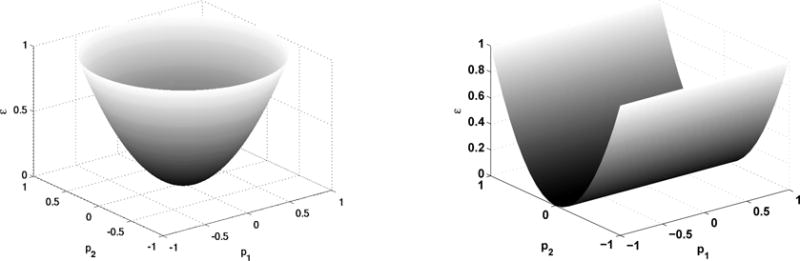
Two minimization functions that may give the same minimum, but very different parameter sensitivities. (a) A paraboloid, and (b) a parabolic cylinder.

Clearly the paraboloid has a well-defined minimum and the slope of the function is the same along all directions in the p₁–p₂ plane. By bending the parabolic cylinder slightly upward along the p₂ axes one can guarantee that the minimimun is at zero, as for the paraboloid, but clearly the sensitivity of the error function with respect to variations in the two parameters is very different. In the remainder of this section we show how scatter plots and sensitivity analysis can be used to detect such differences.

5.1 The use of scatter plots

In this approach one postulates a model, computes the solutions for a wide-range of the parameters, and then compares the difference between the predictions and the experimental results. With first illustrate this with an example of pure diffusion (Model B1) so as to demonstrate the utility as clearly as possible.

The structure of the scatter plots shown in Figure 12 can be understood as follows. When the time interval is short [0,10] the recovery is small and the error is very small for small diffusion coefficients since the error as defined in Figure 5 is the distance between the actual and predicted recovery curves (cf. Figure 13 (right)). When the diffusion coefficient is significantly larger than the true value the predicted recovery curve rises much faster than the true recovery curve and the error increases with the diffusion rate. In an intermediate interval [0,100] the error is significant for both too small and too large a diffusion coefficient. When the observation time period is long [0,1000], the error for larger diffusion coefficients is less significant than for smaller ones because the predicted recovery curve lies close to the true curve at large times, where the error is small (cf. Figure 13 (left)). These results indicate that the intermediate time interval [0,100] is optimal for this problem, since the true diffusion coefficient is most clearly defined at the minimum of the graph of the error.

Figure 12.

Scatterplots of the errors between the model output and the FRAP data versus the diffusion coefficient for different time intervals. The FRAP data is generated by the pure-diffusion model with D = 2.25 × 10⁻⁵ sec⁻¹ to match the data in previous simulations by using the effective diffusion coefficient. The scatterplots are calculated with parameters uniformly distributed on a logarithmic scale D ∈ [1 × 10⁻⁶, 1 × 10⁻³] sec⁻¹. N = 1000 is the number of sample points.

Figure 13.

FRAP recovery data is generated by the pure-diffusion model with D = 2.25 × 10⁻⁵ sec⁻¹. The large D and small D refer to the upper and lower limits of the diffusion coefficients used for the scatterplots, respectively. The figure on the left is plotted on a linear scale, and the one on the right is plotted on a logarithmic scale.

Scatterplots can also give insight for more complicated models such as the diffusion-binding models (Model 1 and Model 2). The top row in Figure 14 shows that the addition of binding to the diffusion-only model of Figure 13 has little effect on the error for a short time interval and small diffusion coefficients, and that the error is dominated by diffusion even for large diffusion coefficients. However the effect of variations in the binding parameters is more pronounced for longer time intervals, but in all cases the role of diffusion remains as shown in Figure 13.

Figure 14.

Scatterplots of the errors between the model output and the FRAP data versus diffusion coefficients and binding affinities for different time intervals. Top and middle panels: FRAP data is generated with D = 2.5 × 10⁻⁴ sec⁻¹, k⁺ = 1 sec⁻¹, k⁻ = 0.1 sec⁻¹. In this and the panels below the parameters are log-uniformly distributed – using D =∈ [1 × 10⁻⁶, 1 × 10⁻³] sec⁻¹, k⁺ ∈ [1 × 10⁻², 10 sec⁻¹], k⁻ ∈ [1 × 10⁻², 10] sec⁻¹. Bottom panel: The FRAP data is generated by the model with diffusion and two binding processes with different rates and affinities D = 2.5×10⁻⁴ sec⁻¹, $k_1^{+}=5{\sec }^{-1}$, $k_1^{-}=0.5{\sec }^{-1}$, $k_2^{+}=0.1{\sec }^{-1}$, $k_2^{-}=5\times {10}^{-3}{\sec }^{-1}$. The parameters are log-uniformly distributed: D ∈ [1 × 10⁻⁶, 1 × 10⁻³] sec⁻¹, k⁺ ∈ [5 × 10⁻³, 5] sec⁻¹, k⁻ ∈ [5 × 10⁻³, 5] sec⁻¹. N = 1000 is the number of sample points for all.

The center row of Figure 14 displays the scatter plots as a function of the binding affinity k⁺/k⁻, for which the true value is 10. For the short time interval T = [0,10] the recovery is small and the effect of diffusion on the error is negligible for large affinities because the fluorescent molecules are tightly bound in the unbleached region and the flux into the bleached region is small. When the binding affinity is small, the influx is larger and diffusion plays a larger role, which leads to larger errors. As the observation time period increases, the difference between these two upper limits diminishes. When the observation time period is long enough, e.g. T ∈ [0, 1000], the situation is reversed. Therefore, using a scatterplot for variable observation times T will suggest what the true affinity is when a T that produces the pattern of errors similar to that in the first figure in the middle panel is found.

These two rows suggest that the scatterplots of errors against diffusion coefficient with different observation time periods identify whether the parameters are located in effective-diffusion regime and if so, what the effective diffusion co-efficient is. If in effective-diffusion regime, by combining the scatterplots against binding affinity and diffusion coefficient, the binding affinity and the effective diffusion coefficient, and thereby the true diffusion coefficient can be obtained.

The bottom row in Figure 14 shows scatterplots of the errors for a one-site recovery model when the true model has two binding sites. These scatterplots with different observation time periods not only can provide the experimentalists with the binding affinities but also can suggest how many different types of binding sites are involved when they have different binding affinities. A binding process with affinity equal to ∼ 10 appears at the scatterplot with the observation time period T ∈ [0, 10]. And the other one with affinity equal to ∼ 20 appears at the scatterplot with T ∈ [0, 100]. Although in reality it may be hard to tell the exact values of binding affinities, the scatterplots with different observation time periods at least help indicate the possiblity of multiple binding sites. They only suggest how many types of binding sites with significantly different rates and affinities are involved.

5.2 Variance-based sensitivity analysis

The scatter-plot-based procedure in the preceding section gives qualitative information about parameters, but more precise tests to determine where the parameter sensitivity lies can be applied after parameter estimation using other methods of sensitivity analysis. The objective of this analysis is to obtain insight as to how the E varies with parameter variation in a neighborhood of the computed minimum. The non-local analysis described below is more informative than simply computing the derivatives of E at the minimum because parameters can be varied over large intervals around the minimum. Here we use a form of variance-based sensitivity for models given in the form Y = f(X₁, X₂, … X_k), where Y is a model output and X₁, X₂, … X_k are factors with respect to which the sensitivity of the output is to be determined (Saltelli et al. 2008; Saltelli et al. 2010). In applying the general technique to the FRAP problem we define $Y=\mathcal{E}$, the error between the observed and predicted recovery as defined earlier, and the factors X are the parameters that are estimated from the data. Thus the model equation is rewritten as

$$\mathcal{E}=f(p_1,p_2,\dots p_k)=f(P),$$ (5.1)

where P = (p₁, p₂, … p_k). For the purpose of the sensitivity analysis that follows we assume that parameters are distributed uniformly.

The first measure of sensitivity is called the first-order sensitivity index of p_i on $\mathcal{E}$, and is obtained as follows. The law of total variance states that

$$V(\mathcal{E})=V_{p_i}(E_{P~i}(\mathcal{E}|p_i))+E_{p_i}(V_{P~i}(\mathcal{E}|p_i)),$$ (5.2)

where V (·) is the variance and P_∼i indicates that the expectation of the variance is taken with respect to all but the i^th parameter. Thus $E_{P~i}(\mathcal{E}|p_i))$ is the expected value of $\mathcal{E}$ that results from averaging over all but p_i. To remove the dependency on the fixed value of p_i, we take the variance with respect to p_i, and after re-arrangement obtain

$$S_i=\frac{V_{p_i}(E_{P~i}(\mathcal{E}|p_i))}{V(\mathcal{E})}=1-\frac{E_{p_i}(V_{P~i}(\mathcal{E}|p_i))}{V(\mathcal{E})}.$$ (5.3)

This measures the contribution of parameter p_i to the total variance, and since it is normalized, it lies in [0, 1]. A large S_i indicates that the parameter p_i contributes a large fraction of the total variance, and thus can be regarded as an important parameter in setting the error. For an additive model, ${\displaystyle {\sum }_{i=1}^k{S}_i=1}$, while for a non-additive model the first order terms do not add up to one, and higher-order interactions amongst the parameters account for some of the variance. For example, if we describe the parabolic cylinder as $p_1^2+p_2^2$, then there is no interaction between the parameters and Σ S_i = 1. This is not the case in the typical FRAP recovery problem, for while the kinetic parameters are independent in the governing evolution equations, their effects on the recovery data are not, since they become conflated in the eigenvalues that determine the time course of recovery. Thus the first-order sensitivities will generally sum to less than one.

A second measure of sensitivity is obtained as follows (Saltelli et al. 2008). The total variance can also be written

$$V(\mathcal{E})=V_{p_i}(E_{P~i}(\mathcal{E}|p_i))+V_{P~i}(E_{p_i}(\mathcal{E}|p_{~i}))+V_{p_i,P~i}$$

wherein the last term accounts for the variance due to the interactions. If the parameter p_i contributes little to the total variance then the sum of the first and last terms is approximately zero, which means that

$$V(\mathcal{E})~V_{P~i}(E_{p_i}(\mathcal{E}|P_{~i}))$$

Thus an alternate measure of a parameter’s effect is the total order sensitivity index of p_i on $\mathcal{E}$, which is defined as

$$S_{Ti}=1-\frac{V_{P~i}(E_{p_i}(\mathcal{E}|P_{~i)}))}{V(\mathcal{E})}=\frac{E_{P~i}(V_{p_i}(\mathcal{E}|P_{~i}))}{V(\mathcal{E})}$$

From the first equality one sees that S_Ti is the expected variance due to the first and higher order effects of p_i on E. For the following simulations the first and total order indices are calculated by using the method of Sobal’ which costs (k + 2)N model runs, where k is the number of parameters and N is the number of sample points in parameter space. N = 1000 is used for all our simulations. The detailed implementation is described in Appendix A.6.

As we showed previously, the FRAP recovery data generated by a theoretical model can be fit very well with a reduced model in some circumstances. For instance, data generated by a diffusion-binding model can be described with a pure-diffusion model when the binding process is much faster than diffusion as shown in the left panel of Figure 15. We proposed that changing the balance between different processes by changing the size of the bleaching region gives rise to a different recovery curve and helps to detect missing processes and to formulate a more appropriate model. When all the processes in the model that generates FRAP data are balanced, i.e., they all occur on comparable time scales, it is unlikely to fit the data with a reduced simple model, as shown in the center panel of Figure 15.

Figure 15.

FRAP data is generated with the intermediate (theoretical) model (Model 2 in Table 1) with the unbalanced processes (left) and the balanced processes (center and right). The true values of the parameters for the unbalanced processes are D = 2.5 × 10⁻⁴ sec⁻¹, k⁺ = 1 × 10⁻¹ sec⁻¹, k⁻ = 5 × 10⁻² sec⁻¹, k^d = 2 × 10⁻³ sec⁻¹, and the parameters for the balanced processes are D = 2.5 × 10⁻⁴ sec⁻¹, k⁺ = 1 × 10⁻² sec⁻¹, k⁻ = 5 × 10⁻³ sec⁻¹, k^d = 2 × 10⁻³ sec⁻¹. Parameters are estimated by using the simple (recovery) model (Model B2 in Table 1, which is also the same as that in (Kicheva et al. 2007)) for the left and center panels, and using the complex (recovery) model (Model A.33 in Appendix) in the right panel. The estimates are (left) D = 7.8322 × 10⁻⁶ sec⁻¹, k_d = 1.2698 × 10⁻³ sec⁻¹; (center) D = 7.0290 × 10⁻⁶ sec⁻¹, k_d = 9.9313 × 10⁻⁴ sec⁻¹; (right) D = 4.4680 × 10⁻⁴ sec⁻¹, k⁺ = 1.7633 sec⁻¹, k⁻ = 1.1396 × 10⁻¹ sec⁻¹, kⁱ = 1.1131 × 10⁻², k^o = 6.0198 × 10⁻³ sec⁻¹, k_t = 1.7574 × 10⁻⁷ sec⁻¹, k_d1 = 2.1856 × 10⁻³ sec⁻¹, k_d2 = 1.1563 × 10⁻³ sec⁻¹.

However, when a complex model that includes more processes than are important is used to fit the data, it may be difficult to detect this from the fit of the recovery curve. As shown in the right panel of Figure 15, even though all the processes in the intermediate model that generates the data are well balanced, we can still fit the data very well with a complex model, and this is where the sensitivity analysis can be useful. In this case, when the sensitivity analysis is implemented using the intermediate (theoretical) model, the sensivity indices of all the parameters are comparable, and none of the total indices is very small. However, when the sensitivity analysis is applied to the complex model, the total-order indices of some parameters, such as k^t and k^d2 shown in (c) and (d) of Figure 16. This suggests the possibility of over-parameterization, i.e., the more detailed model might include non-influential processes that are not detectable using the available data.

Figure 16.

FRAP data is generated with the intermediate model (Model 2 in Table 1) with parameters D = 2.5 × 10⁻⁴ sec⁻¹, k⁺ = 1 × 10⁻² sec⁻¹, k⁻ = 5 × 10⁻³ sec⁻¹, k^d = 2 × 10⁻³ sec⁻¹. (a) and (b): The first order and total order sensitivity indices are calculated by using the same intermediate model with parameters with uniform linear distribution D ∈ [0.5×10⁻⁵, 4.5×10⁻⁵] sec⁻¹, k⁺ ∈ [0.2 × 10⁻², 1.8 × 10⁻²] sec⁻¹, k⁻ ∈ [1 × 10⁻³, 9 × 10⁻³] sec⁻¹, k^d ∈ [0.4 × 10⁻³, 3.6 × 10⁻³] sec⁻¹. (c) and (d): The first order and total order sensitivity indices are calculated by using the complex model A.33 with parameters with uniform linear distribution around the estimates ([0.2 × Estimate, 1.8 × Estimate]) D ∈ [0.8510 × 10⁻⁴, 7.6594 × 10⁻⁴] sec⁻¹, k⁺ ∈ [0.3526, 3.1739] sec⁻¹, k⁻ ∈ [0.2849 × 10⁻¹, 2.5641 × 10⁻¹] sec⁻¹, kⁱ ∈ [0.2226 × 10⁻², 2.0036 × 10⁻²] sec⁻¹, k^o ∈ [1 × 10⁻³, 9 × 10⁻³] sec⁻¹, k^t ∈ [0.3515 × 10⁻⁷, 3.1633 × 10⁻⁷] sec⁻¹, k^d1 ∈ [0.3868 × 10⁻³, 3.4816 × 10⁻³] sec ⁻¹, k^d2 ∈ [0.2313 × 10⁻³, 2.0813 × 10⁻³] sec⁻¹.

It is worth noting that when parameters are estimated using either the reduced simple model (Kicheva et al. 2007) or the complex model (Zhou et al. 2012) with the same FRAP data generated by the intermediate model, estimates of diffusion coefficients in both recovery models (4.26×10⁻⁴ sec⁻ vs. 1.41×10⁻⁶ sec⁻) differ by a factor of 60, which is similar to the large difference in the measurement of the diffusion coefficient of Dpp in (Kicheva et al. 2007) and (Zhou et al. 2012). However, in our simulations, neither of the estimates are close to the true value for data generation even though two models can fit the steady-state (results not shown here) and recovery data.

6 Discussion

In an experimental context the standard approach to use the FRAP technique is to measure the experimental data and then fit a model to the recovery curve. While informative, it is difficult to analyze the model and evaluate the quality of estimates because the parameters underlying physical processes in reality are unknown. Our aim here was to approach this problem by using a theoretical model to generate FRAP data and postulating a recovery model to estimate the parameters, and knowing both a priori enabled us to quantitatively assess the quality of estimates and find ways to improve them. Firstly, by using a recovery model identical to the theoretical model, we showed that good fitting of the data may be misleading in some circumstances, in that it does not always indicate high quality estimates. We identified factors that lead to poor parameter estimation from FRAP data, and suggested three new, feasible ways in which the estimation can be improved - using the FRAP data in an appropriate observation time period, changing the size of the bleaching region to rebalance the diffusion and kinetic processes, and using the spatial information of FRAP data. Then, by varying the recovery model from the theoretical model, we showed that a simplified recovery model can adequately describe the FRAP processes in some circumstances, and established the relationship between parameters in the theoretical model and those in the recovery model. Finally, we introduced variance-based parameter sensitivity into FRAP analysis, and suggested that the important kinetic processes might be detected by sensitivity analysis before estimation, and the over-parameterization problem in a FRAP model can be perceived by doing sensivity analysis after estimation.

In using FRAP, it is important to determine which processes should be included in the recovery model. For example, ignoring binding processes that are present in the system may lead to underestimation of the diffusion coefficient by an order of magnitude. Given FRAP data, we proposed two different ways that can facilitate identification of the appropriate model. We found that changing the size of the bleaching region gives rise to different FRAP recovery curves and can provide insight into the relative effects of diffusion and binding kinetics. In particuar, reducing the size of the bleaching region to speed up the diffusion process relative to the kinetic processes can help uncover a hidden binding process in the recovery curve, which might be neglected when the bleaching region is large. In addition, we showed that preliminary sensitivity analysis using scatterplots with physically reasonable ranges of parameters may also help detect multiple binding processes. Using the two methods will reduce the chance of neglecting important processes in the model. In addition, sensitivity analysis after estimation using the first and total order indices can suggest over-parameterization problem in a FRAP model, i.e., the model contains non-influential processes. If some of the parameters have very low total-order indices, the model is more complex than is justified by the data available, and has to be reduced by eliminating the non-influential processes. This step can be repeated until none of the parameters in the model have extremely low total-order indices. The ideal scenario is that the corresponding sensitivity index around the estimate of each parameter in the model is comparable, which indicates all the processes are well balanced. Incorporating these methods into the FRAP analysis can greatly increase the probability of formulating appropriate models and thereby also increase the accurary of parameter estimation.

Although we showed that reducing the size of the bleaching region can help to formulate a more appropriate model and improve parameter estimation in some circumstances, it is difficult to decide what the size of the bleaching region should be at the outset of a FRAP experiment. However the knowledge of the effect of a reduction can be used in the following way. After the estimates of parameters are obtained from a first FRAP experiment, one can calculate the characteristic time scales of diffusion and kinetic processes, and depending on the results, the experiment can be re-done with a bleaching region that leads to a better balance of the processes. Similar remarks apply to the use of spatial information in FRAP data. Averaging spatial FRAP data over the whole bleaching region looses some information which might be useful for parameter estimation. However, for a realistic FRAP experiment, the spatial FRAP data always contains noise which is greatly tenuated by averaging FRAP data. We suggest that it is possible to benefit from spatial FRAP data if local averaging rather than global averaging is implemented. In addition to the quality of parameter estimation, the advantage of using spatial FRAP data may be explored in many other aspects of model identification, such as estimation of more parameters in FRAP models.

In summary, we suggest that the procedure shown in Figure 17 to better use FRAP data in the process of model formulation and parameter estimation. This method can be used for general FRAP modeling and analysis not discussed here. For instance, the assumptions used here, such as an instantaneous and homogeneous bleaching process, may not be valid in some circumstances, and it would be interesting to apply our method to model the whole FRAP processes as described in Appendix A.3, and to study how different assumptions affect the estimates quantitatively.

Figure 17.

A suggested procedure for improving model identification and parameter estimation.

The establishment of the morphogen profiles in the wing disc is a very complex process that may involve several distinct morphogen transport processes, endo- and exocytosis of the morphogen, and intracellular sequestration of it. As a result, parameter estimates derived from fitting of FRAP recovery curves are not likely to bear a close relationship to true parameter values, since the FRAP data is inadequate to extract the true parameters in a complex model. Thus such tissue-level applications of FRAP must be supplemented with other techniques in order to identify the processes and the attendant parameters. This remains as a significant challenge in the context of developmental biology.

The simple model described by (2.16) has been used to estimate parameters from experimental FRAP data in several systems, but it may have very limited applicability in identifying the parameters that govern the in vivo dynamics, since other kinetic or transport processes are usually involved. Even in the simple case of Bicoid dynamics in the early Drosophila embryo, processes other than diffusion and reaction, including binding, localization of Bicoid in the nuclei, and non-homogeneities in the cytosol and cortical layer of the syncytium, are certainly involved. Moreover, in a cellularized system such as the Drosophila wing disc there may be several other modes of cell-cell communication.

The complexity involved in the interactions of multiple transport processes with binding, internalization and kinetic transformation is hidden by analyzing the spread of morphogens using a simple reaction-diffusion system such as (2.16), and how one relates the ‘real’ parameters in individual steps to parameters in such a high-level description is usually difficult to determine analytically. This has lead to dramatic differences (cf. (Kicheva et al. 2007; Zhou et al. 2012) in the estimates of parameters for a simplified description such as (2.16), and raises the question as to what those parameters represent.

Table 7.

Spatial FRAP improves parameter estimation as much as reducing the size of the bleaching region does.

True values of parameters			Bleaching size	Observation T	Estimates of parameters
D	k+	k−	Method	T (sec)	D	k+	k−
2.5e-4	1	0.1	Default	1000	1.8661e-4	0.7167	9.9335e-2
				100	1.9132e-4	0.7542	0.1013
				10	2.5689e-4	0.9684	0.09649
			Reduced size	100	2.4228e-4	0.9666	0.09999
				10	2.4364e-4	0.9666	0.09990
			Spatial FRAP	1000	2.5411e-4	1.0176	9.9956e-2
				100	2.5397e-4	1.0169	0.09995
				10	2.5093e-4	1.004	0.09992

Table 11.

Parameter estimation in reduced models when there are multiple binding sites.

Theoretical Model (Model 2)							Reduced Model (Model 1)
Diffusion + Two binding sites					Bleaching size	Time	Diffusion + Single binding site			Curve fitting
D	$k_1^{+}$	$k_1^{-}$	$k_2^{+}$	$k_2^{-}$	δ−	T (sec)	D	k+	k−
2.5e-4	1	0.1	10	1	Default	100	2.2629e-5	8.2322e-2	9.2352e-2	good
2.5e-4	1e-3	1e-3	10	1	Default	1000	2.2122e-5	8.4915e-5	9.8877e-4	good
2.5e-5	1e-3	1e-3	1	0.1	Default Reduce Size	1000 1000	2.2413e-6 1.1746e-6	1.3014e-4 6.2724e-1	1.3478e-3 1.5113	good bad

Table 12.

Parameter estimation in reduced models when there is diffusion, binding, internalization, decay and influx in the theoretical model. The data is generated using Model 4 with parameters D = 2.5 × 10⁻⁴ sec⁻¹, k⁺ = 1 sec⁻¹, k⁻ = 0.1 sec⁻¹, kⁱ = 2.6 × 10⁻³ sec⁻¹, k^d = 1 × 10⁻² sec⁻¹. The flux J is fixed during parameter estimation.

	Theoretical Model	Reduced Model (Model 3)	Reduced Model (Model B2)
D	2.5e-4	4.54e-5	1.51e-5
k+	1	3.38e-2
k−	0.1	2.28e-2
ki	2.6e-3
kd	0.01	3.19e-3	1.85e-3

A Appendix

A.1 The general framework

The general form of the system of reaction-diffusion equations that we shall use hereafter have the following form.

$$\frac{\partial c}{\partial t}=D_c{\nabla }^{2}c+\overline{R}(c,\overline{p})\mathrm{in}\mathrm{\Omega }$$ (A.1)

$$\mathbf{n}\cdot D_c\nabla c=\overline{J}\text{on}\partial \mathrm{\Omega }$$ (A.2)

$$c(r,0)=c_0(r),$$ (A.3)

Here the vector c = (c₁, c₂, ⋯, c_m) is the vector of chemical concentrations, D_c is assumed to be a constant diagonal matrix, and J is a prescribed flux on∂Ω. Ω is a bounded region in ℜ^q, q = 1, 2 with a smooth boundary and outward normal n. The functions ${\overline{R}}_i$ give the net rate of production of the i^th species and they are herein are always linear or quadratic polynomials in the c_i’s. The vector $\overline{p}$ is a parameter vector, which can include the kinetic constants and perhaps species that appear in the kinetic mechanism but do not change significantly on the time scale of interest. As described in the preceding example, we can regard these equations as appropriate for a thin fluid layer over a 1D or 2D domain. In applications to the wing disc the geometry of the hexagonal packing of cells is more complex than the description above and a mathematical description that accounts for the geometric complexity is far more complex. A 2D model of the disc that incorporates this complexity is given in (Umulis and Othmer 2014).

This system can be nondimensionalized as follows. Let L be a measure of the size of the system, C_i be a reference concentration for species i, and ω⁻¹ be a time scale characteristic of the reactions⁷. Define the dimensionless quantities u_i = c_i/C_i, τ = ωt, D_i = D_ci/ωL², and ξ = r/L, where r ≡ (x₁, ⋯, x_q). The dimensionless governing equations are

$$\begin{array}{ll}\frac{\partial u}{\partial \tau }=D{\nabla }^{2}u+R(u,p)\hfill & \text{in}\mathrm{\Omega }\hfill \\ \mathbf{n}\cdot D\nabla u=J\hfill & \text{on}\partial \mathrm{\Omega }\hfill \\ u(\xi ,0)=u_0(\xi )\hfill & \hfill \end{array}$$ (A.4)

where D = diag{D₁, D₂, ⋯, D_m}, $J_i={\overline{J}}_i/(\omega C_i)$, R(u, p) is the dimensionless form of $\overline{R}(c,\overline{p})$, and Ω is scaled. If there are species that do not diffuse the corresponding D_i and J_i are zero, and unless stated otherwise, we assume that all boundary fluxes are zero, i.e., we impose homogeneous Neumann boundary conditions.

We show later that in many FRAP experiments the kinetics can be linearized, and therefore in the majority of what follows we focus on linear kinetic models, and we write the system (A.4) as

$$\begin{array}{r}\frac{\partial u}{\partial \tau }=D{\nabla }^{2}u+Ku\\ \mathbf{n}\cdot \nabla u=0,\text{on}\partial \mathrm{\Omega }\\ u(\xi ,0)=u_0(\xi )\end{array}$$ (A.5)

This system has solutions of the form

$$u(\xi ,\tau )={\displaystyle \sum _{n=0}^{\infty }{y}_n(\tau ){\varphi }_n}$$ (A.6)

where ϕ_n is a solution of the scalar eigenvalue problem

$$\begin{array}{l}{\nabla }^2{\varphi }_n=-{\alpha }_n^2{\varphi }_n\\ \mathbf{n}\cdot \nabla {\varphi }_n=0\end{array}$$ (A.7)

and y_n is given by

$$y_n(\tau )=e^{(K-{\alpha }_n^{2}D)\tau }{y}_n(0).$$ (A.8)

For a reasonable boundary the eigenfunctions ϕ_n form a complete orthonornal set under the standard L₂ inner product [u, v] = ∫ u(ξ)v(ξ)dξ, and the solution of (A.5) can be written as (Othmer and Scriven 1969)

$$u(\xi ,\tau )={\displaystyle \sum _{n=0}^{\infty }{e}^{(K-{\alpha }_n^{2}D)\tau }{y}_n(0){\varphi }_n(\xi .)}$$ (A.9)

The initial condition can be written

$$u_0(\xi )={\displaystyle \sum _{n=0}^{\infty }{y}_n(0){\varphi }_n(\xi )}$$ (A.10)

and therefore y_n(0) = 〈u₀(ξ), ϕ_n〉, where here and hereafter 〈·, ·〉 denotes the real or complex, as appropriate, Euclidean inner product, taken component-wise when one argument is a vector and the other a scalar.

Remark 2

If the influx is non-zero, i.e., J ≠ 0, we let w = u − u^s where u^s is the steady state solution. Then w satisfies

$$\frac{\partial w}{\partial \tau }=D{\nabla }^{2}w+Kw$$ (A.11)

with zero Neumann boundary conditions. The solution w has the representation given at (A.9), and u is obtained from this. In particular, when m = 1, we obtain the solution given at (2.17).

The difficulty in FRAP analysis of multicomponent systems, even when they are linear, stems from the structure of (A.9). To simplify the analysis, suppose that the family of matrices $\{K-{\alpha }_n^{2}D\}$ is semisimple – which means that they can be diagonalized – for all n. Then the matrix exponential has the representation

$$e^{(K-{\alpha }_n^{2}D)\tau }={\displaystyle \sum _{j=1}^m{e}^{{\mathrm{\lambda }}_{\mathit{jn}}\tau }{P}_{\mathit{jn}}}$$ (A.12)

where the projections P_jn are associated with a given λ_jn (Kato 1966). Since we assume that the $\{K-{\alpha }_n^{2}D\}$ are semisimple they have the representation

$$P_{\mathit{jn}}={\mathrm{\Psi }}_{\mathit{jn}}\ast {\mathrm{\Psi }}_{\mathit{jn}}^{\ast }$$ (A.13)

wherein Ψ_jn is an eigenvector of $K-{\alpha }_n^{2}D$ associated with λ_jn and ${\mathrm{\Psi }}_{\mathit{jn}}^{\ast }$ is the corresponding adjoint eigenvector. The action of any P on a vector u is defined by

$$Pu=\langle {\mathrm{\Psi }}_{\mathit{jn}}^{\ast },u\rangle {\mathrm{\Psi }}_{\mathit{jn}}.$$

The eigenvector Ψ_jn = (Ψ_1jn, ⋯, Ψ_mjn)^T ∈ ℜ^m is a solution of the algebraic eigenvalue problem

$$\begin{array}{lll}(K-{\alpha }_n^{2}D-{\mathrm{\lambda }}_{\mathit{jn}}I){\mathrm{\Psi }}_{\mathit{jn}}=0,\hfill & j=1,2,\cdots ,m,\hfill & n=0,1,\dots \hfill \end{array}.$$ (A.14)

and the eigenvalues λ_jn are solutions of the characteristic equation

$$\mathit{det}(K-{\alpha }_n^{2}D-\mathrm{\lambda }I)=0.$$ (A.15)

The problem simplifies significantly when K and D commute, for then the eigenvalues of $K-{\alpha }_n^{2}D$ are simply ${\mathrm{\lambda }}_{\mathit{jn}}={\mathrm{\lambda }}_j^K-{\alpha }_n^2{\mathrm{\lambda }}_j^D$.

The characteristic equation is an m^th degree polynomial for an m-component system. Thus, while the representation at (A.12) has the apparently simple form of a sum of exponentials, the eigenvalues λ_jn and the eigenfunctions Ψ_jn are complicated functions of the kinetic rate parameters and the diffusion constants. The case m = 1 is as done previously, and only if m = 2 or 3 can one make analytical progress toward understanding how the eigenvalues and eigenfunctions depend on the rate parameters (Othmer and Scriven 1969), and only in these cases can one hope to gain analytical insights into the problem of extracting rate parameters from FRAP data. We turn to these cases in the following sections.

If R(u, p) = Ku + F (u, ξ, τ) the general solution of (A.4) can be written as

$$u(\xi ,\tau )={\displaystyle {\int }_{\mathrm{\Omega }}G(\xi -\xi \prime ,\tau )u_0(\xi \prime )d\xi \prime +{\displaystyle {\int }_0^t{\displaystyle {\int }_{\mathrm{\Omega }}G(\xi ,\xi \prime ,\tau -\tau \prime )F(u,\xi ,\tau \prime )d\xi \prime d\tau \prime }}}$$ (A.16)

where G(ξ, ξ^′, t) is the Green’s function for the linear operator L = D∇² + K. This has the representation

$$G(\xi -\xi \prime ,\tau -\tau \prime )={\displaystyle \sum _{n=0}^{\infty }{\displaystyle \sum _{j=1}^m{e}^{{\mathrm{\lambda }}_{\mathit{jn}}(\tau -\tau \prime )}{P}_{\mathit{jn}}{\varphi }_n(\xi ){\varphi }_n(\xi \prime )}}$$ (A.17)

This form (A.16) can be used when diffusion during bleaching and waiting periods are incorporated in the analysis.

A.2 A special case – diffusion and binding only

The general framework allows for first-order reactions of any type (of which there are four –cf. (Gadgil et al. 2005)), but when the only processes are diffusion of the fluorescent species and binding to one or more independent immobile sites more can be said about the solutions. Suppose there are m − 1 independent types of binding sites, as shown in Figure 18. In Appendix A.4 we re-derive the known fact (Sprague et al. 2004) that for a single binding site the recovery process can be modeled as a linear process, even though the binding step is nonlinear, and point out that the on- and off-rates in the resulting equations are composites of parameters in the original equations (Sprague et al. 2004). The analysis given there can be applied to the case of m − 1 independent types of binding sites, although the amount of unbound fluorescent molecules is the solution of a higher-order polynomial when there is more than one type of site. This leads to the linear system

$$\begin{array}{l}\frac{\partial u_1}{\partial \tau }=D{\nabla }^2{u}_1-{\displaystyle \sum _{k=2}^m{B}_k(u_1,u_k,\tau )}\text{for}\xi \in (0,1)\\ \frac{d{u}_k}{d\tau }=B_k(u_1,u_k,\tau )\equiv k_{k1}{u}_1-k_{1k}{u}_{k}k=2,\cdots ,m\\ u(\xi ,0)=u_0(\xi )\end{array}$$ (A.18)

Thus the matrices K and D in (A.5) take the following form.

$$K=\left[\begin{array}{ccccc}-{\displaystyle {\sum }_{j=2}^m{k}_{j1}}& k_{12}& k_{13}& \cdots & k_{1m}\\ k_{21}& -k_{12}& 0& \cdots & 0\\ ⋮& & & & \\ k_{m1}& 0& 0& \cdots & -k_{1m}\end{array}\right]$$ (A.19)

and D = diag(D₁, 0, 0, ⋯, 0). The columns of the matrix K sum to zero and therefor K is singular, and if the k_ij are all non-zero it is irreducible and an application of the Perron-Froebenius theorem shows that the zero eigenvalue is simple. The fact that the kinetic steps are mass-preserving implies that the left eigenvector of K corresponding to the zero eigenvalue is (1, 1, 1, ⋯, 1)^T, and therefore

$$\frac{\partial }{\partial \tau }(u_1+u_2+\cdots +u_m)=D_1{\nabla }^2{u}_1,$$ (A.20)

which reflects the fact that the total local concentration only changes due to diffusion.

Figure 18.

The notation for m-1 binding sites

The matrix K can be symmetrized, and therefore the eigenvalues are all real and non-positive. The kinetic interactions involved in binding are restricted to the reaction simplex defined by the relation ${\displaystyle {\sum }_{i=1}^m{u}_i(t)}={\displaystyle {\sum }_{i=1}^m{u}_i(0)}$. The foregoing properties of K also imply that there is a unique steady state of the equation

$$\frac{\mathit{du}}{d\tau }=Ku$$

on the simplex defined by the initial condition. Eq. (A.20) shows how the simplices vary in space due to diffusion, but two useful extreme cases arise when either diffusion is slow relative to the binding or when it is rapid relative to binding. The first case arises when either the on-rate or the off-rate of every binding step is large relative to ${\tau }_D^{-1}=D_1/L^2$. Then a singular-perturbation analysis shows that to leading order in the small parameter ε ≡ τ_R/τ_D, the kinetics reach the steady state on the reaction simplex defined by the initial data at every point in space, and these simplices then evolve slowly on the diffusion time scale.

In this limit the free and bound forms are related by

$$u_i=\frac{k_{i1}}{k_{1i}}{u}_1\equiv K_i{u}_1,i=2,\cdots ,m.$$ (A.21)

to within correction terms proportional to ε.⁸ As a result, (A.20) becomes

$$\frac{\partial }{\partial \tau }(1+{\displaystyle \sum _{i=2}^m{K}_i})u_1=D_1{\nabla }^2{u}_1$$ (A.22)

which leads to a diffusion equation for u₁ with the effective diffusion coefficient

$$D_{1,\mathit{eff}}=\frac{D_1}{1+{\displaystyle {\sum }_{i=2}^m{K}_i}}$$ (A.23)

This reduction of the diffusion coefficient in the presence of rapid binding was apparently first observed by Crank (Crank 1975).

When τ_D ≪ τ_R, i.e., D₁/L² is much larger than the largest kinetic rate constant, one can show that to lowest order the spatial distribution of fluorescent molecules relaxes to a uniform state given by

$${\overline{u}}_1(\xi ,t)~{\overline{u}}_1(0)-{\displaystyle \sum _{k=2}^m{\displaystyle {\int }_0^t\overline{B_k}(u_1,u_k,\tau )d\tau }}$$ (A.24)

where the overbar denotes the spatial average and $\overline{B_k}(u_1,u_k,\tau )\equiv k_i^{+}{\overline{u}}_1-k_i^{-}{\overline{u}}_i$. This solution can then be used in the binding equations to obtain an explicit expressions for the ${\overline{u}}_k(\tau ),k=2,\cdots ,m$. Thus the evolution on the slow time scale is simply the readjustment of the fractions of bound fluorescent molecules. Since the diffusion time scale depends on the length scale of the domain, the balance between diffusion and binding can be controlled by altering the size of the bleaching region.

A.3 A summary of the FRAP protocol

The setup and the sequence of steps in a typical FRAP experiment that uses a confocal laser scanning microscope (CLSM) are as follows, and assuming that diffusion is the only transport process, the steps are modeled as shown below which also explains Figure 1. We describe them in generality here, and detailed descriptions of the models used for parameter estimation are given later. Both bleaching and scanning steps are done pixel by pixel and line by line.

Step 1: Prebleaching

Use a low intensity laser to scan the fluorescence density in the entire domain Ω which includes the ROI. The evolution of the concentrations of fluorescent molecules during the pre-bleaching time [0, T₀] (cf. Fig. 1) is governed by

$$\frac{\partial c}{\partial t}=D{\nabla }^{2}c+R(c)-I_{p}c$$

where R(c) represents the reaction processes, and I_p is the pre-bleaching function. The pre-bleaching process is usually modeled as a first-order process as above, and in a 2D domain the intensity is given by

$$I_p(t,x,y)=I_{p_0}\mathit{exp}\left(-\frac{2\left[{\left(x-X(t)\right)}^2+{\left(y-Y(t)\right)}^2\right]}{r_0^2}\right),$$

wherein x = X(t), y = Y (t) and x, y ∈ Ω describes the pre-bleaching path of the laser.

Step 2: Bleaching

Use a high intensity beam to bleach the ROI for an interval of length T₁. In this phase

$$\frac{\partial c}{\partial t}=D{\nabla }^{2}c+R(c)-Ic$$

with initial conditions obtained from the end of the pre-bleaching period. The differences between pre-bleaching and bleaching are the laser intensity and pixel dwell time for scanning, as well as the scanning domain.

Step 3: Postbleaching

This usually comprises a waiting time T₂ between the end of bleaching and the beginning of observation. During the observation time use a low intensity beam to image the fluorescence recovery process. During the waiting time

$$\frac{\partial c}{\partial t}=D{\nabla }^{2}c+R(c)$$

with initial conditions obtained from the end of step 2.

During the observation period T₃

$$\frac{\partial c}{\partial t}=D{\nabla }^{2}c+R(c)-I_{p}c$$

with initial conditions obtained from the end of the waiting period.

The inconsistencies in FRAP partly from different assumptions for models. One of the disparate assumptions lie in that of initial conditions for recovery phase, the obtainment of which can be divided into two categories among existing FRAP models. The first one is modeling all the previous processes before recovery phase to get the initial conditions (Kang et al. 2009; Braeckmans et al. 2007; Braeckmans et al. 2003; Mazza et al. 2008). By modeling the pre-bleaching, bleaching and recovery phase, the analytical solution representing FRAP data can be derived in some special occasions and with certain assumptions (Braeckmans et al. 2003). It provides us insights about how the bleaching process and others affect the FRAP recovery, however, it requires prior knowledge of some parameters to model activities of the laser beam. Another way which is more popular to estimate parameters is to only model the recovery phase with assumptions about the initial conditions which can be obtained by the first post-bleach image of fluorescence. In this category, there are three different kinds of assumptions which all neglect the bleaching effect with imaging process in recovery phase. One natural assumption is the piece-wise constant initial conditions from direct measurement of the size of the photobleaching spot (Sprague et al. 2004). This is validated when the bleaching is homogeneous and the bleaching time is negligible. Another one is also the piece-wise constant initial conditions but are deduced from the final recovery concentration and the conservation of fluorescence (Hinow et al. 2006). It is an improvement from the first one, but still is limited to the cases where the boundaries of the bleached region are relatively sharp and the observational photobleaching is negligible. When the boundaries of the bleached region is smoothed by diffusion before observation, the piece-wise constant is not able to capture the characteristics of the initial condition, which may cause large errors in parameter estimation (Mueller et al. 2008). Thus for the third kind, some Gaussian or Gaussian-edge function fitted by the initial data, which results from the Gaussian assumption of the laser profile, is used for the initial condition (Mueller et al. 2008). It has been shown that using the Gaussian expression of the initial post-bleach profile alter the estimates of parameters in comparison to the first or second utilization of initial condition, however, the utilization of Gaussian function needs to be carefully justified. It is not convincing that the utilization of Gaussian function as the initial condition produces better estimations, because in real biological system the true values of binding/unbinding rates as well as the diffusion coefficient are unknown. In our simulations, we only simulate the data without with homogenous and instantaneous bleaching process, and thus we estimate parameters by only modeling the recovery with piece-wise constant initial conditions.

A.4 Justification of the assumption of linear kinetics in FRAP modeling

Suppose that there is one diffusing species that can bind to an immobile receptor, and let (u₁, v₁) and (u₂, v₂) be the free and bound concentrations of fluorescent and bleached molecules, respectively. These satisfy the following equations.

$$\begin{array}{c}\frac{\partial u_1}{\partial \tau }=D_1{\nabla }^2{u}_1-k^{+}{u}_1[R]+k^{-}{u}_2\\ \frac{\partial u_2}{\partial \tau }=k^{+}{u}_1[R]-k^{-}{u}_2\end{array}$$ (A.25)

$$\begin{array}{c}\frac{\partial u_1}{\partial \tau }=D_1{\nabla }^2{v}_1-k^{+}{v}_1[R]+k^{-}{v}_2\\ \frac{\partial v_2}{\partial \tau }=k^{+}{v}_1[R]-k^{-}{v}_2\end{array}$$ (A.26)

where [R] is the concentration of free binding sites.

The sums w₁ = u₁ + v₁ and w₂ = u₂ + v₂ satisfy

$$\frac{\partial w_1}{\partial \tau }=D_1{\nabla }^2{w}_1-k^{+}{w}_1[R]+k^{-}{w}_2$$ (A.27)

$$\frac{\partial w_2}{\partial \tau }=k^{+}{w}_1[R]-k^{-}{w}_2.$$ (A.28)

If adequate time has elapsed before bleaching begins, one can assume that the system is at steady state prior to bleaching, and further assume that bleaching does not perturb the binding reactions, it merely substitutes a bleached for a fluorescent molecule. Then throughout the bleaching process $w_1=w_1^s$, the steady-state value of the free concentration, and the total free concentration of binding sites is given by

$$R=R_T\frac{\widehat{K}}{\widehat{K}+w_1^s},$$ (A.29)

where R_T = R + w₂ is the total concentration (free and occupied) of binding sites and $\widehat{K}=k^{-}/k^{+}$. Similarly, the concentration of bound sites is

$$w_2^s=R_T\frac{w_1^s}{\widehat{K}+w_1^s}.$$

Let W = w₁ + w₂ be the total concentration of all forms of the molecules, which here is assumed constant pointwise in space and time. Then it follows that $w_1^s$ is the solution of a quadratic equation whose coefficients involve K, W and R_T, and the solution of this quadratic then leads to the free site concentration (A.29), and (A.25) can be written as

$$\begin{array}{l}\frac{\partial u_1}{\partial \tau }=D_1{\nabla }^2{u}_1-k^{+}{u}_1+k^{-}{u}_2\\ \frac{\partial u_2}{\partial \tau }=k^{+}{u}_1-k^{-}{u}_2\end{array}$$ (A.30)

where $k^{+}=k^{+}([R_T]-w_2^s)$ and k⁻ = k⁻. This is the linear system widely-used in this context, and that data what data is used to estimate the co-efficients involved. However, the constant k⁺ is a composite constant the involves three separate constants in an experiment, and two other independent measurements are needed to determine the three independent constants.

To define the initial conditions, let I₀(ξ) = u₁₀(ξ) + u₂₀(ξ) be the initial concentration of the fluorescent molecules in space at the onset of the recovery phase of an experiment, which is usually measured directly from the first postbleaching image. If we assume that bleaching in the ROI is instantaneous (i.e., T₁ = 0), then the initial condition for equation (A.30) is

$$\begin{array}{ccc}{u}_{10}=\frac{I_0(\xi )}{1+K_d^{-1}}& \text{and}& u_{20}=\frac{I_0(\xi )}{1+K_d}\end{array}.$$

where K_d ≡ k⁻/k⁺ is the dissociation constant. In the simulations described in the text these are piecewise constant functions. If bleaching is not instantaneous then diffusion alters the initial condition, and the initial conditions for the recovery period must be computed using the equations applicable to the interval [T₀, T₀ + T₁] given in Section A.3.

A.5 Analysis of the eigenvalues and eigenvector for a two-component system

In the following, we use eigenvalues/eigenvectors to analyze how FRAP data is determined by the parameters in the model.

Let

$$Q=K-{\alpha }_n^{2}D=\left(\begin{array}{cc}-k^{+}-{\alpha }_n^2{D}_1& k^{-}\\ k^{+}& -k^{-}\end{array}\right)$$

and

$$\gamma =k^{+}-k^{-}+{\alpha }_n^2{D}_1$$

Then the eigenvalues of the matrix Q are:

$$\begin{array}{c}{\mathrm{\lambda }}_{1n}=-\frac{1}{2}(k^{+}+k^{-}+{\alpha }_n^2{D}_1)+\sqrt{{\gamma }^2+4k^{+}{k}^{-}})\\ {\mathrm{\lambda }}_{2n}=-\frac{1}{2}(k^{+}+k^{-}+{\alpha }_n^2{D}_1)-\sqrt{{\gamma }^2+4k^{+}{k}^{-}})\\ {\mathrm{\lambda }}_{10}=-(k^{+}+k^{-}),{\mathrm{\lambda }}_{20}=0.\end{array}$$

The averaged fluorescent intensity can be written as

$$\overline{u_1}+\overline{u_2}\equiv \left(\overline{u_{10}}+\overline{u_{20}}\right)+{\displaystyle \sum _{n=1}^{\infty }g(n)\left(\overline{u_{1n}}+\overline{u_{2n}}\right)}=y_{10}+y_{20}+{\displaystyle \sum _{n=1}^{\infty }g(n)\left(d_{1n}{e}^{{\mathrm{\lambda }}_{1n}t}+d_{2n}{e}^{{\mathrm{\lambda }}_{2n}t}\right)}$$ (A.31)

where

$$\begin{array}{l}{u}_{10}=\frac{k^{+}{y}_{10}-k^{-}{y}_{20}}{k^{+}+k^{-}}{e}^{{\mathrm{\lambda }}_{10}t}+\frac{k^{-}{y}_{10}+k^{-}{y}_{20}}{k^{+}+k^{-}}\\ u_{20}=\frac{k^{-}{y}_{20}-k^{+}{y}_{10}}{k^{+}+k^{-}}{e}^{{\mathrm{\lambda }}_{10}t}+\frac{k^{+}{y}_{10}+k^{+}{y}_{20}}{k^{+}+k^{-}}\end{array}$$

(thus, u₀ + u₂₀ = y₁₀ + y₂₀)

$$g(n)=\frac{1}{n(l_R-l_L)\pi }\left[\mathit{sin}(n\pi l_R)-\mathit{sin}(n\pi l_L)\right]$$

Note that

$$\begin{array}{c}{\mathrm{\lambda }}_{1n}{\mathrm{\lambda }}_{2n}={\alpha }_n^2{D}_1{k}^{-}\\ d_{1n}=\frac{y_{1n}+y_{2n}}{2}-\frac{{\alpha }_n^2{D}_1(y_{2n}-y_{1n})}{2\sqrt{{\gamma }^2+4k^{+}{k}^{-}}}-\frac{(k^{+}+k^{-})(y_{1n}+y_{2n})}{2\sqrt{{\gamma }^2+4k^{+}{k}^{-}}}\\ d_{2n}=\frac{y_{1n}+y_{2n}}{2}+\frac{{\alpha }_n^2{D}_1(y_{2n}-y_{1n})}{2\sqrt{{\gamma }^2+4k^{+}{k}^{-}}}+\frac{(k^{+}+k^{-})(y_{1n}+y_{2n})}{2\sqrt{{\gamma }^2+4k^{+}{k}^{-}}}\end{array}$$

since

$$\begin{array}{c}{y}_{10}+y_{20}=\frac{1}{N}{\displaystyle \sum _{k=1}^N{I}_0(k)}\\ y_{1n}+y_{2n}=\frac{1}{N}{\displaystyle \sum _{k=1}^N{I}_0(k)(\mathit{cos}\frac{n\pi }{N}(k-1)+\mathit{cos}\frac{n\pi }{N}k)}\end{array}$$

Note that it is positive and independent of the parameters

$$y_{2n}-y_{1n}=\frac{k^{+}-k^{-}}{k^{+}+k^{-}}\frac{1}{N}{\displaystyle \sum _{k=1}^N{I}_0(k)(\cos \frac{n\pi }{N}(k-1)+\cos \frac{n\pi }{N}k)=\frac{k^{+}-k^{-}}{k^{+}+k^{-}}(y_{1n}+y_{2n})}$$

If we define

$$f(n)=g(n)\frac{y_{1n}+y_{2n}}{2}$$

we have

$$\overline{u_1}+\overline{u_2}=\frac{1}{N}{\displaystyle \sum _{k=1}^N{I}_0(k)+}{\displaystyle \sum _{n=1}^{\infty }f(n)(c_{1n}{e}^{{\mathrm{\lambda }}_{1n}t}+c_{2n}{e}^{{\mathrm{\lambda }}_{2n}t})}$$ (A.32)

where

$$\begin{array}{l}{c}_{1n}=1-\frac{{\alpha }_n^2{D}_1\frac{k^{+}-k^{-}}{k^{+}+k^{-}}}{\sqrt{{\gamma }^2+4k^{+}{k}^{-}}}-\frac{k^{+}+k^{-}}{\sqrt{{\gamma }^2+4k^{+}{k}^{-}}}\\ c_{2n}=1+\frac{{\alpha }_n^2{D}_1\frac{k^{+}-k^{-}}{k^{+}+k^{-}}}{\sqrt{{\gamma }^2+4k^{+}{k}^{-}}}+\frac{k^{+}+k^{-}}{\sqrt{{\gamma }^2+4k^{+}{k}^{-}}}\end{array}$$

Note that c_1n, c_2n > 0, λ_1n, λ_2n < 0.

As n increases, c_1n increases, c_2n decreases, both λ_1n and λ_2n decrease (algebraically).

Moreover, as n → ∞, ${\mathrm{\lambda }}_{1n}\to -{\alpha }_n^2{D}_1$, λ_2n → −k⁻, and if k⁺ > k⁻,

$$c_{1n}\to 2\frac{k^{-}}{k^{+}+k^{-}},c_{2n}\to 2\frac{k^{+}}{k^{+}+k^{-}}$$

if k⁺ < k⁻,

$$c_{1n}\to 2\frac{k^{+}}{k^{+}+k^{-}},c_{2n}\to 2\frac{k^{-}}{k^{+}+k^{-}}$$

and if k⁺ = k⁻,

$$c_{1n}\to 1,c_{2n}\to 1.$$

One may first estimate the eigenvalues and corresponding eigenvectors from FRAP data based on equation (A.32). Then by the relationship between unknown paramters and eigenvalues and eigenvectors, targeted diffusion coefficient and kinetic parameters may be eventually estimated. Moreover, the quantitative analysis of eigenvalues may lead to some more insight of parameter estimation. These aspects can be explored in the future.

A.6 Implementation of sensitivity analysis

The indices of variance-based sensitivity measures are usually done by the Monte Carlo Method. In practice, instead of generating pseudo-randomly distributed points in the parameter space in traditional Monte Carlo Method, the low-discrepancy quasi-random number generator is used to improve the efficiency of the estimators. This is known as the Quasi-Monte Carlo method. It is implemented as follows (taken from (Saltelli et al. 2010)).

1. “Generate an N ×2k sample matrix with respect to the probability distributions of the input variables- the parameters. N is the number of sample points. k is the dimension of parameter space, i.e., the number of parameters.

2. Use the first k columns of the matrix as matrix A, and the remaining k columns as matrix B, which generates two independent samples of N points in the k-dimensional parameter space

3. Build k further N × k matrices $A_B^i$ for i = 1, 2, …, k, such that the ith column of $A_B^i$ is equal to the ith column of B, and the remaining columns are from A

4. The A, B, and the k $A_B^i$ matrices specify N × (k + 2) points in the parameter space (one for each row). Run the model at each point, giving a total of N × (k + 2) model evaluations, i.e., the corresponding f(A), f(B) and $f(A_B^i)$ values

5. Calculate the sensitivity indices using the estimators discussed below.”

There are a number of Monte Carlo estimators for both indices. Two that are currently widely used are according to the rule proposed by Saltelli et al. (2010).

$$\begin{array}{l}{V}_{p_i}(E_{P~i}(\mathcal{E}|p_i)\approx \frac{1}{N}{\displaystyle \sum _{j=1}^{N}f{(B)}_j(f{(A_b^i)}_j-f{(A)}_j)}\\ E_{X~i}{\left(V_{p_i}\left(\mathcal{E}|p_{~i}\right)\approx \frac{1}{2N}{\displaystyle \sum _{j=1}^N(f{\left(A_b^i\right)}_j-f{\left(A\right)}_j}\right)}^2\end{array}$$

They are used for the estimation of S_i and S_Ti respectively.

A.7 The complex model used in Section 5.2

$$\begin{array}{c}\frac{\partial u_1}{\partial \tau }=D_1{\nabla }^2{u}_1-k^{+}{u}_1+k^{-}{u}_2\\ \frac{\partial u_2}{\partial \tau }=k^{+}{u}_1-k^{-}{u}_2-k^i{u}_2+k^o{u}_3\\ \frac{\partial u_3}{\partial \tau }=-k^i{u}_2-k^o{u}_3-k^t{u}_3-k^{d1}{u}_3\\ \frac{\partial u_4}{\partial \tau }=-k^t{u}_3-k^{d2}{u}_4\end{array}$$ (A.33)

References

- Amonlirdviman K, Khare NA, Tree DR, Chen WS, Axelrod JD, Tomlin CJ. Mathematical modeling of planar cell polarity to understand domineering nonautonomy. Science. 2005;307(5708):423–6. doi: 10.1126/science.1105471. [DOI] [PubMed] [Google Scholar]
- Beaudouin J, Mommer Mario S, Bock Hans Georg, Eils Roland. Pages 157–169 of: 22 Model Based Parameter Estimation. Springer; 2013. Experiment Setups and Parameter Estimation in Fluorescence Recovery After Photobleaching Experiments: A Review of Current Practice. [Google Scholar]
- Braeckmans K, Peeters L, Sanders NN, De Smedt SC, Demeester J. Three-dimensional fluorescence recovery after photobleaching with the confocal scanning laser microscope. Biophysical journal. 2003;85(4):2240–2252. doi: 10.1016/s0006-3495(03)74649-9. [DOI] [PMC free article] [PubMed] [Google Scholar]
- Braeckmans K, Remaut K, Vandenbroucke RE, Lucas B, De Smedt SC, Demeester J. Line FRAP with the confocal laser scanning microscope for diffusion measurements in small regions of 3-D samples. Biophysical journal. 2007;92(6):2172–2183. doi: 10.1529/biophysj.106.099838. [DOI] [PMC free article] [PubMed] [Google Scholar]
- Crank J. The mathematics of Diffusion. Oxford; Claredon Press: 1975. [Google Scholar]
- Driever W, N?sslein-Volhard C. The bicoid protein determines position in the Drosophila embryo in a concentration-dependent manner. Cell. 1988;54(1):95–104. doi: 10.1016/0092-8674(88)90183-3. [DOI] [PubMed] [Google Scholar]
- Driever W, Nüsslein-Volhard C. A gradient of bicoid protein in Drosophila embryos. Cell. 1988;54(1):83–93. doi: 10.1016/0092-8674(88)90182-1. [DOI] [PubMed] [Google Scholar]
- Gadgil C, Lee CH, Othmer HG. A stochastic analysis of first-order reaction networks. Bull Math Biol. 2005;67:901–946. doi: 10.1016/j.bulm.2004.09.009. [DOI] [PMC free article] [PubMed] [Google Scholar]
- Goentoro LA, Reeves GT, Kowal CP, Martinelli L, Schpbach T, Shvartsman SY. Quantifying the Gurken morphogen gradient in Drosophila oogenesis. Dev Cell. 2006;11:263–272. doi: 10.1016/j.devcel.2006.07.004. [DOI] [PMC free article] [PubMed] [Google Scholar]
- Grimm O, Coppey M, Wieschaus E. Modelling the Bicoid gradient. Development. 2010;137(14):2253. doi: 10.1242/dev.032409. [DOI] [PMC free article] [PubMed] [Google Scholar]
- Hinow P, Rogers CE, Barbieri CE, Pietenpol JA, Kenworthy AK, DiBenedetto E. The DNA binding activity of p53 displays reaction-diffusion kinetics. Biophysical journal. 2006;91(1):330–342. doi: 10.1529/biophysj.105.078303. [DOI] [PMC free article] [PubMed] [Google Scholar]
- Kang M, Day CA, Drake K, Kenworthy AK, DiBenedetto E. A generalization of theory for two-dimensional fluorescence recovery after photobleaching applicable to confocal laser scanning microscopes. Biophysical journal. 2009;97(5):1501–1511. doi: 10.1016/j.bpj.2009.06.017. [DOI] [PMC free article] [PubMed] [Google Scholar]
- Kato T. Perturbation Theory for Linear Operators. Springer-Verlag; 1966. [Google Scholar]
- Kicheva Anna, Pantazis Periklis, Bollenbach Tobias, Kalaidzidis Yannis, Bittig Thomas, Julicher Frank, Gonzalez-Gaitan Marcos. Kinetics of morphogen gradient formation. Science. 2007;315(5811):521–525. doi: 10.1126/science.1135774. [DOI] [PubMed] [Google Scholar]
- Lander Arthur D. Morpheus unbound: reimagining the morphogen gradient. Cell. 2007;128(2):245–256. doi: 10.1016/j.cell.2007.01.004. [DOI] [PubMed] [Google Scholar]
- Mai J, Trump S, Ali R, Schiltz LR, Hager G, Hanke T, Lehmann I, Attinger S. Are assumptions about the model type necessary in reaction-diffusion modeling? a frap application. Biophysical journal. 2011;100(5):1178–1188. doi: 10.1016/j.bpj.2011.01.041. [DOI] [PMC free article] [PubMed] [Google Scholar]
- Mazza D, Braeckmans K, Cella F, Testa I, Vercauteren D, Demeester J, De Smedt SS, Diaspro A. A new FRAP/FRAPa method for three-dimensional diffusion measurements based on multiphoton excitation microscopy. Biophysical journal. 2008;95(7):3457–3469. doi: 10.1529/biophysj.108.133637. [DOI] [PMC free article] [PubMed] [Google Scholar]
- Mueller F, Wach P, McNally JG. Evidence for a common mode of transcription factor interaction with chromatin as revealed by improved quantitative fluorescence recovery after photobleaching. Biophysical journal. 2008;94(8):3323–3339. doi: 10.1529/biophysj.107.123182. [DOI] [PMC free article] [PubMed] [Google Scholar]
- Müller P, Rogers KW, Jordan BM, Lee JS, Robson D, Ramanathan S, Schier AF. Differential diffusivity of nodal and lefty underlies a reaction-diffusion patterning system. Science. 2012;336(6082):721–724. doi: 10.1126/science.1221920. [DOI] [PMC free article] [PubMed] [Google Scholar]
- Müller P, Rogers KW, Shuizi RY, Brand M, Schier AF. Morphogen transport. Development. 2013;140(8):1621–1638. doi: 10.1242/dev.083519. [DOI] [PMC free article] [PubMed] [Google Scholar]
- Orlova DY, Bártová E, Maltsev VP, Kozubek S, Chernyshev AV. A nonfitting method using a spatial sine window transform for inhomogeneous effective-diffusion measurements by frap. Biophysical journal. 2011;100(2):507–516. doi: 10.1016/j.bpj.2010.11.080. [DOI] [PMC free article] [PubMed] [Google Scholar]
- Othmer HG, Scriven LE. Interactions of reaction and diffusion in open systems. Ind and Eng Chem Fund. 1969;8:302–315. [Google Scholar]
- Othmer Hans G, Painter Kevin, Umulis David, Xue Chuan. The intersection of theory and application in biological pattern formation. Math Mod Nat Phenom. 2009;4:3–79. doi: 10.1051/mmnp/20094401. [DOI] [PMC free article] [PubMed] [Google Scholar]
- Perkins TJ, Jaeger J, Reinitz J, Glass L. Reverse engineering the gap gene network of Drosophila melanogaster. PLoS Comput Biol. 2006;2(5):0417–28. doi: 10.1371/journal.pcbi.0020051. [DOI] [PMC free article] [PubMed] [Google Scholar]
- Reeves GT, Muratov CB, Schupbach T, Shvartsman SY. Quantitative models of developmental pattern formation. Dev Cell. 2006;11(3):289–300. doi: 10.1016/j.devcel.2006.08.006. [DOI] [PubMed] [Google Scholar]
- Saltelli A, Annoni P, Azzini I, Campolongo F, Ratto M, Tarantola S. Variance based sensitivity analysis of model output. Design and estimator for the total sensitivity index. Computer Physics Communications. 2010;181(2):259–270. [Google Scholar]
- Saltelli Andrea, Ratto Marco, Andres Terry, Campolongo Francesca, Cariboni Jessica, Gatelli Debora, Saisana Michaela, Tarantola Stefano. Global sensitivity analysis: the primer. John Wiley & Sons; 2008. [Google Scholar]
- Seiffert Sebastian, Oppermann Wilhelm. Systematic evaluation of frap experiments performed in a confocal laser scanning microscope. Journal of microscopy. 2005;220(1):20–30. doi: 10.1111/j.1365-2818.2005.01512.x. [DOI] [PubMed] [Google Scholar]
- Serpe M, Umulis D, Ralston A, Chen J, Olson DJ, Avanesov A, Othmer H, O’Connor MB, Blair SS. The BMP-binding protein Crossveinless 2 is a short-range, concentration-dependent, biphasic modulator of BMP signaling in Drosophila. Dev Cell. 2008 Jun;14:940–953. doi: 10.1016/j.devcel.2008.03.023. [DOI] [PMC free article] [PubMed] [Google Scholar]
- Shvartsman SY, Muratov CB, Lauffenburger DA. Modeling and computational analysis of EGF receptor-mediated cell communication in Drosophila oogenesis. Development. 2002;129:2577–2589. doi: 10.1242/dev.129.11.2577. [DOI] [PubMed] [Google Scholar]
- Spirov A, Fahmy K, Schneider M, Frei E, Noll M, Baumgartner S. Formation of the bicoid morphogen gradient: an mRNA gradient dictates the protein gradient. Development. 2009 Feb;136:605–614. doi: 10.1242/dev.031195. [DOI] [PMC free article] [PubMed] [Google Scholar]
- Sprague BL, Pego RL, Stavreva DA, McNally JG. Analysis of Binding Reactions by Fluorescence Recovery after Photobleaching. Biophys Jour. 2004;86(6):3473–3495. doi: 10.1529/biophysj.103.026765. [DOI] [PMC free article] [PubMed] [Google Scholar]
- Sprague BL, McNally JG. Frap analysis of binding: proper and fitting. Trends in cell biology. 2005;15(2):84–91. doi: 10.1016/j.tcb.2004.12.001. [DOI] [PubMed] [Google Scholar]
- Turing AM. The chemical basis of morphogenesis. Phil Trans R Soc Lond B. 1952;237:37–72. doi: 10.1098/rstb.2014.0218. [DOI] [PMC free article] [PubMed] [Google Scholar]
- Umulis D, O’Connor MB, Othmer HG. Robustness of embryonic spatial patterning in Drosophila melanogaster. Curr Top Dev Biol. 2008;81:65–111. doi: 10.1016/S0070-2153(07)81002-7. [DOI] [PMC free article] [PubMed] [Google Scholar]
- Umulis DM, Serpe M, O’Connor MB, Othmer HG. Robust, bistable patterning of the dorsal surface of the Drosophila embryo. Proc Natl Acad Sci. 2006;103(31):11613–8. doi: 10.1073/pnas.0510398103. [DOI] [PMC free article] [PubMed] [Google Scholar]
- Umulis David M, Othmer Hans G. The Role of Mathematical Models in Understanding Pattern Formation in Developmental Biology. Bulletin of Mathematical Biology. 2014:1–29. doi: 10.1007/s11538-014-0019-7. [DOI] [PMC free article] [PubMed] [Google Scholar]
- Wolpert L. Positional information and the spatial pattern of cellular differentiation. J Theor Biol. 1969;25:1–47. doi: 10.1016/s0022-5193(69)80016-0. [DOI] [PubMed] [Google Scholar]
- Yakoby N, Bristow CA, Gouzman I, Rossi MP, Gogotsi Y, Schpbach T, Shvartsman SY. Systems-level questions in Drosophila oogenesis. Syst Biol (Stevenage) 2005;152:276–284. doi: 10.1049/ip-syb:20050039. [DOI] [PubMed] [Google Scholar]
- Zhou Shaohua, Lo Wing-Cheong, Suhalim Jeffrey L, Digman Michelle A, Gratton Enrico, Nie Qing, Lander Arthur D. Free Extracellular Diffusion Creates the Dpp Morphogen Gradient of the Drosophila Wing Disc. Current Biology. 2012;22(8):668–675. doi: 10.1016/j.cub.2012.02.065. [DOI] [PMC free article] [PubMed] [Google Scholar]