Resolution of Students t-tests, ANOVA and analysis of variance components from intermediary data

Abstract

Significance testing in comparisons is based on Student’s t-tests for pairs and analysis of variance (ANOVA) for simultaneous comparison of several procedures. Access to the average, standard deviation and number of observations is sufficient for calculating the significance of differences using the Student’s tests and the ANOVA. Once an ANOVA has been calculated, analysis of variance components from summary data becomes possible. Simple calculations based on summary data provide inference on significance testing. Examples are given from laboratory management and method comparisons. It is emphasized that the usual criteria of the underlying distribution of the raw data must be fulfilled.

Introduction

Comparison of results from different experimental designs, between instruments and between methods is an everyday task in analytical chemistry and its applied sciences, e.g. laboratory medicine. Usually, statistical inference is based on original observations fed into statistical packages that deliver the requested statistics. The obvious procedure is to start with inspecting the raw data to determine the appropriate statistical methods to be used. However, sometimes the raw data may not be available whereas the central tendency (e.g. the average), the dispersion (e.g. the standard deviation) and the number of observations may be. Yet, it may be desirable to evaluate the significance of a difference between datasets. Typical situations may be related to laboratory management and scientific evaluation of reports. We describe how this can be accomplished if the datasets are independent and fulfil the requirements of Student’s t-test or analysis of variance (ANOVA). Resolution of an ANOVA table to provide analysis of variance components is particularly discussed.

Methods

Student’s t-test

There are two Student’s t-tests; one evaluates pairs of results with something in common, known as the dependent test, t_dep. The other compares the averages of independent results, t_ind.

A classic example of a dependent design is comparing the results obtained from the same individuals before and after a treatment. An independent design would be, for instance, comparing the results obtained in groups of healthy men and women. Thus, the t_dep considers the difference between every pair of values, whereas the t_ind only considers the averages, the standard deviation and number of observations in each group. Access to these intermediary quantities allows calculating the t-value.

To further understand the difference between the t-values and the formal prerequisites and conditions for their use, it may be helpful to consider how they are calculated.

The t_dep considers the differences between paired measurements and is calculated by the different but equivalent formats of the Equation 1 (Eq.1):

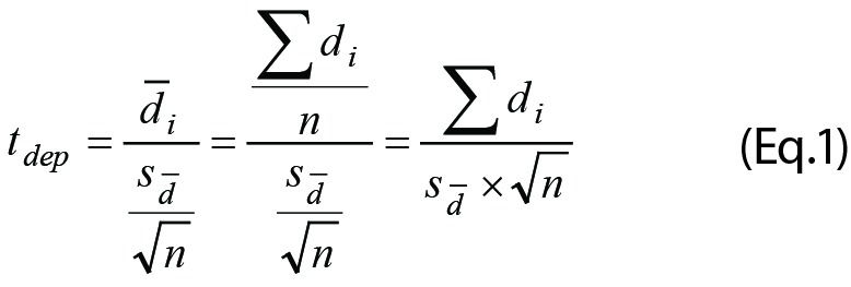If expressed in words, t_dep is the average of the differences between observations, , divided by its standard error 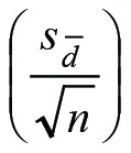.. Rearrangement of Eq.1 may facilitate calculations. The degrees of freedom, df, is n-1.

The differences shall be normally distributed. If that distribution is far from normal then using the t_dep cannot be justified and a non-parametric test should be applied, e.g. the Wilcoxon test.

The t_dep is limited to comparing two sets of dependent individual data, e.g. results before and after an intervention. The datasets must be of equal sizes but need not be normally distributed. If the parameters of Eq.1 are known, i.e. the average difference between pairs and their standard error of the mean, then t_dep can be calculated without direct access to the original results. It is unlikely that results of a comparison are reported in this way and the intermediary calculation of t_dep does not have a given place in the arsenal.

Student’s t_ind from intermediary data

Access to the average, standard deviation and number of observations but not the original observations allows evaluating the significance of the difference; i.e. when results are presented with only information about the central tendency and data dispersion. Provided the original datasets can be assumed to be normally distributed the significance (t_ind) of a difference between the averages can be estimated according to Equation 2 (Eq.2).

The t_ind considers the difference between the averages of two datasets in relation to the square root of the sum of their respective squared standard error of the mean.

This standard calculation may be less known or recognized in the era of calculators and statistical packages. The averages and standard deviations are calculated or otherwise available from the original data sets and then entered into Eq.2. If the number of observations in the groups is similar and the standard deviations of the same magnitude, the degrees of freedom, df, is n₁ + n₂ – 2.

Consider, for instance, that the cholesterol concentration of two groups of healthy men from widely different environments was reported as the averages, standard deviation and number of observations (Table 1). The calculated t_ind using Eq.2 was:

Table 1. Results of cholesterol concentration measurements in two groups of men.

	Group 1	Group 2
Average	5.0	4.4
Standard deviation	1.4	1.3
F-value	1.16
Number of observations	100	100

Although we do not know for certain if the original results were normally distributed – and independent – this may be a reasonable assumption considering that the averages and standard deviations of the data were originally provided.

The variances were compared and evaluated by an F-test and found not significantly different. Thus, the df = 100 + 100 – 2 = 198.

The significance of a t-value (however generated) is evaluated by the same t-table which is available in many text books and on the internet (1). The null hypothesis is that there is no difference between the groups. The null hypothesis is discarded if the t-value is above a critical value (usually corresponding to P = 0.05). A calculated t-value can be directly evaluated by the Excel functions T.DIST.2T(t, df) or T.DIST.RT(t, df), the functions referring to a two- or one-tail problem, respectively.

The cholesterol values of the two groups are statistically different with P = 0.002 and P = 0.001 for the two- and one-tail problem, respectively. The “critical value” is obtained by the functions T.INV(probability;df) and T.INV.2T(probability;df) for one and two tail problems, respectively.

The variances of the distributions as well as the difference between their averages are the important quantities in evaluating the difference between the distributions. The variances are assumed to be equal in the estimation of the df. This can be tested using the “F-test”. This test is designed to compare the dispersion (variance) of two datasets with the null hypothesis that there is no difference. The assumption in this case is that one of the variances is larger than the other; this is therefore a one-tailed problem. To fit tables and other calculations the larger of the two variances shall be in the nominator. Consequently, the calculated statistic, the F-value, is always above 1. The farther away from one, the larger is the probability that there is a difference between the variances.

To quantify the probability of a difference between the variances, a table should be consulted but the table data can also be retrieved from Excel.

As an example we can evaluate a possible difference between the variances reported in Table 1.

The probability (P) for a significant difference of the F-value 1.16 is 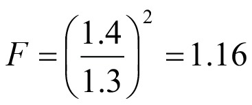. The corresponding probability P = 0.231 (one-tail) is ob-tained using the function F.DIST.RT(x,df1,df2). This should be compared with the critical P-value (P_crit) for the desired significance level and degrees of freedom for the individual datasets using the function F.INV.RT(p,df1,df2). Since P_crit = 1.39, the null hypothesis is not discarded and the variances are equal. The “RT” (right tail) in these functions limits the calculations to a one-tailed situation where only the upper limit of the right skew distribution is considered.

If the F-test reveals that there is a high probability of a significant difference between the variances, then estimating the df according to Welch-Satterthwaite should be considered (2, 3). A detailed discussion of this procedure is outside the scope of the present paper. The calculated df will not always be an integer and since only the df, not the t-value per se is affected, the outcome may only indirectly have an effect on the inference.

Accordingly, however, Excel offers two t_ind procedures, “assuming equal variances” and “unequal variances”. It is safer to always use the latter; if the variances happen to be similar, the t-value and the degrees of freedom are anyway calculated correctly.

If the datasets are not normally distributed, non-parametric procedures should be used, e.g. the Mann-Whitney test.

ANOVA from intermediary results

If a specific quantity of a given sample is measured repeatedly on several occasions, e.g. using different instruments or on different days, it may be interesting to compare the averages in the groups or from the various occasions. The procedure of choice in this case is the ANOVA. The ANOVA reduces the risk of overestimating a significance of differences caused by chance which may be an effect of repeated t_ind.

Since several groups/instruments are studied, observations are repeated in “two directions”, within the groups and between the groups. Consequently, the ANOVA reports the variation within the groups and between the groups.

The ANOVA is calculated from the “sum of squares”, i.e. the differences between observations and their averages, squared. Essentially, this is the same principle as that of calculating the sample variance, i.e. the sum of squares divided by the df (n-1).

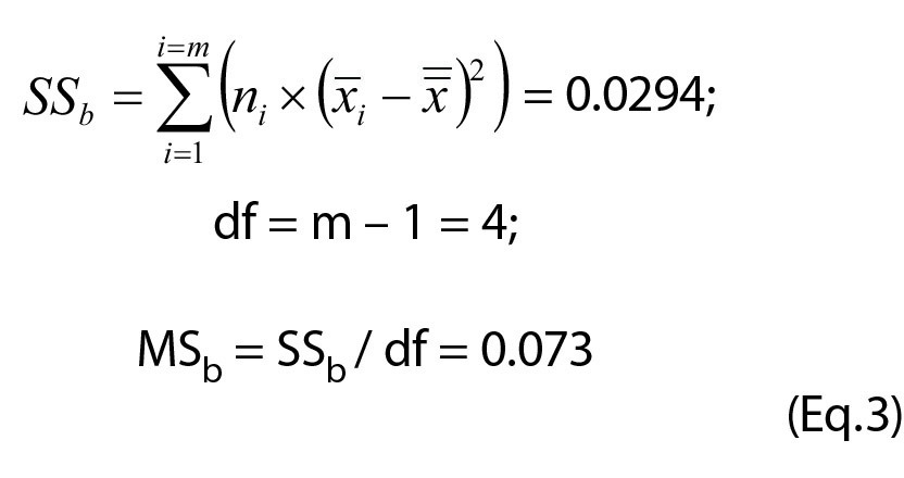
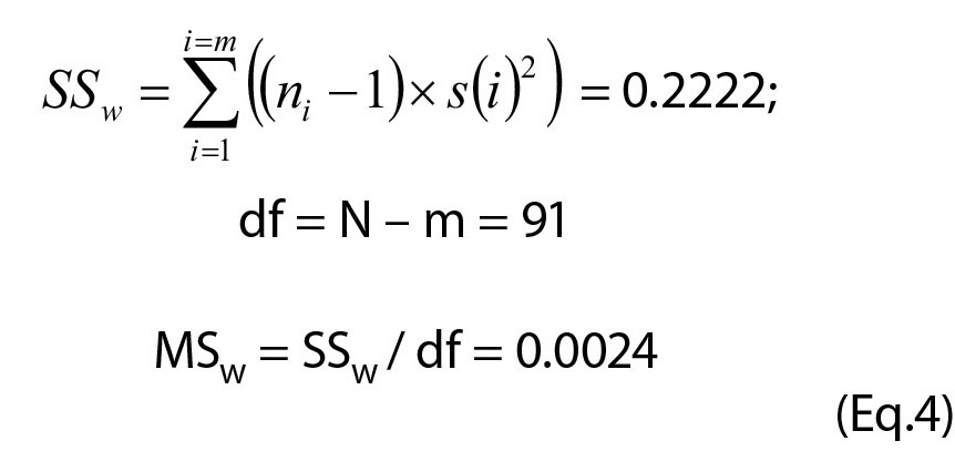
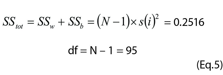
The stepwise resolution of the example in Table 2 is given in Equations 3, 4 and 5 (Eq.3-5), and also summarized in Table 3.

Table 2. Results from repeated measurements of a sample in five different laboratories.

	Lab 1	Lab 2	Lab 3	Lab 4	Lab 5
Number of observations	18	15	24	21	18
Average	1.38	1.37	1.42	1.39	1.40
Standard deviation	0.040	0.050	0.060	0.050	0.040

Table 3. The ANOVA analysis based on data from Table 2.

	df	SS	MS	F - value	P	P0.05
Between	4	0.0294	0.0073	3.01	0.022	2.47
Within	91	0.2222	0.0024
Total	95	0.2516
df – degrees of freedom. SS – sum of squares. MS – mean square.

The following abbreviations are used to describe the calculations involved: SS_b, SS_w and SS_tot represent the sums of squares between groups (SS_b), within groups (SS_w) and total (SS_tot); MS represents the mean square obtained as SS/df; i individual groups, the average of the values in group i, the average of all observations, the standard deviation of the values in group m, m the number of groups, the number of observations in group m and the total number of observations. The symbol Σ is a conventional shorthand symbol, interpreted as the sum of the terms in the adjacent parenthesis.

The Eq. 3 - 5 show that in the calculation of an ANOVA only the averages, variances, and the observations in each group and number of groups are necessary.

The sum of squares may be difficult to visualize but divided by the degrees of freedom the mean squares (MS) are created. These represent the variances within the groups (MS_w) and between the groups (MS_b). However, the latter also includes the variances emanating from the within groups and a correction needs to be considered to estimate the “pure between group variance”. See below Equations 6 and 7 (Eq.6 and 7).

If the null hypothesis H₀: µ₁=µ₂=…=µ_m, is false then MS_b > MS_w and thus the ratio MS_b / MS_w > 1. µ_n represents the true averages of the groups. This ratio can be recognized as an F-test and used to evaluate the difference between the groups. The calculated F-value is evaluated in a common F-table or by Excel function F.DIST.RT(F,df₁,df₂) or F.DIST(F,df₁,df₂,cumulative) and expressed as a probability for the validity of the null hypothesis. Normally, a probability less than 5% (i.e. P < 0.05) is anticipated for statistical significance.

The results of an ANOVA are conventionally reported in a table (Table 3) based on the actual results, Figure 1.

Figure 1.

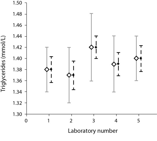
Results from Table 2.
The squares represent the averages, the continuous line the standard deviations, and the dotted error bars the standard error of the mean for each laboratory listed in Table 2.

Analysis of variance components

The ANOVA allows defining the between- (reproducibility) and within- (repeatability) group variances. The key elements of the ANOVA table are the MSs.

The MS_w represents the within group variance whereas the MS_b is a composite measure of the “pure between” and within-group variances. The necessary correction to isolate the pure between-group variance is:

where n is the number of observations in the groups. If the number of observations is the same in every group, the design is “balanced” and n equals the average number of observations in the groups, whereas in an unbalanced design the number of observations differs between the groups and a correction needs to be included:

where N is the total number of observations (2, 4).

However, the correction by subtracting the relative variance of the number of observations over the groups is bound to be small and therefore the average number of observations in the groups is usually appropriate (Table 4).

Table 4. The analysis of variance components.

	Variance	SD	CV, %
Pure between component	0.000255	0.016024	1.1
Ditto adjusted for unbalance	0.000257	0.016024	1.1
Within component	0.002442	0.049414	3.5
Total	0.002697	0.051947	3.7
SD – standard deviation. CV – coefficient of variation. The number of significant digits is exaggerated to visualize the effect of correction for an unbalanced design.

The combined variance is:

This quantity is also called intra-laboratory variance (3). The corresponding intra-laboratory standard deviation is 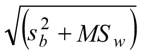. The result of the example in Table 2 is summarized in Table 4.

If the MS_b is smaller than MS_w, their difference (Eq.6) would become negative and the s_b cannot be calculated. In such cases the total variance is conventionally set equal to MS_w.

A total variance can also be calculated directly from all the observations. However, this approach may over- or underestimate the intra-laboratory variance depending on the between- and within group variances.

Discussion

Statistical software may produce results, irrespective of the validity of the input data, or put another way, the chosen statistical procedure may not be “fit for purpose”. It is therefore necessary to understand what is going on “behind the scene”. As a bonus, procedures to estimate some test quantities without access to the original data become available. This may have practical consequences in laboratories’ comparisons of results, particularly using Student’s independent t tests, ANOVA and Analysis of variance components. The same limitations regarding normality and equal variances will apply as when using raw data but since the input data, particularly the standard deviation, already require normality this is usually not a major issue. The intermediate calculation of an ANOVA may be justified since the results of repeated measurements of a particular quantity will vary randomly. This also applies to the situation when the same sample is measured repeatedly in different laboratories. The use of the “Analysis of variance components” procedure can be of great help in finding the root cause to impaired quality of measurements (2, 4, 5). The use of intermediary data may be particularly useful in managing the quality of conglomerates of laboratories where access to summary data would allow simple calculation of within- and between laboratory imprecision and eventually a fair appreciation of the total imprecision.

References

- 1.NIST/SEMATECH e-Handbook of Statistical Methods Available at: http://www.itl.nist.gov/div898/handbook/prc/section4/prc44.htm. Accessed February 2nd 2017.
- 2.Kallner A, editor. Laboratory statistics. 1st ed. Waltham, MA: Elsevier Inc., 2014. [Google Scholar]
- 3.Clinical and Laboratory Standards Institute (CLSI). User verification of precision and estimation of bias. CLSI document EP15 3A. 3rd ed. Wayne, PA: CLSI, 2014. [Google Scholar]
- 4.Armitage P, Berry G, Matthews JSN, editors. Statistical methods in medical research. 4th ed. Malden, MA: Blackwell Science Ltd., 2008. [Google Scholar]
- 5.Cardinal RN. Graduate-level statistics for psychology and neuroscience. Available at https://egret.psychol.cam.ac.uk/psychology/graduate/Guide_to_ANOVA.pdf. Accessed February 2nd 2017.