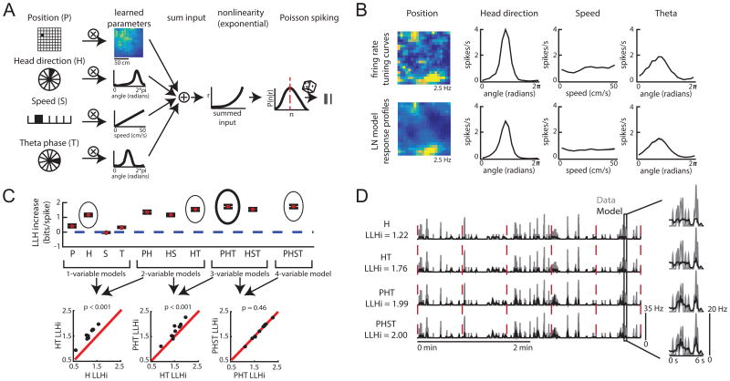
Figure 2.

The LN model provides an unbiased method for quantifying neural coding. A. Schematic of LN model framework. P, H, S and T are binned into 400, 18, 10, and 18 bins, respectively. The filled bin denotes the current value, which is projected (encircled x) onto a vector of learned parameters. This is then put through an exponential nonlinearity that returns the mean rate of a Poisson process from which spikes are drawn. B. Example firing rate tuning curves (top) and model-derived response profiles (bottom, computed from the PHST model; means from 30 bootstrapped iterations shown in black and the standard deviation in gray). C. Top: Example of model performance across all models for a single neuron (mean ± SEM log- likelihood increase in bits, normalized by the number of spikes [LLHi]). Selected models are circled, with the final selected model in bold. Bottom: comparison of selected models. Each point represents the model performance for a given fold of the cross-validation procedure. The forward-search procedure identifies the simplest model whose performance on held-out data was significantly better than any simpler model (p < 0.05). D. Comparison of the cell's firing rate (gray) with the model predicted firing rate (black) over 4 minutes of test data. Model type and model performance (LLHi) listed on the left. Red lines delineate the 5 segments of test data. Firing rates were smoothed with a Gaussian filter (o = 60 ms). (See also Figures S1 and S2)