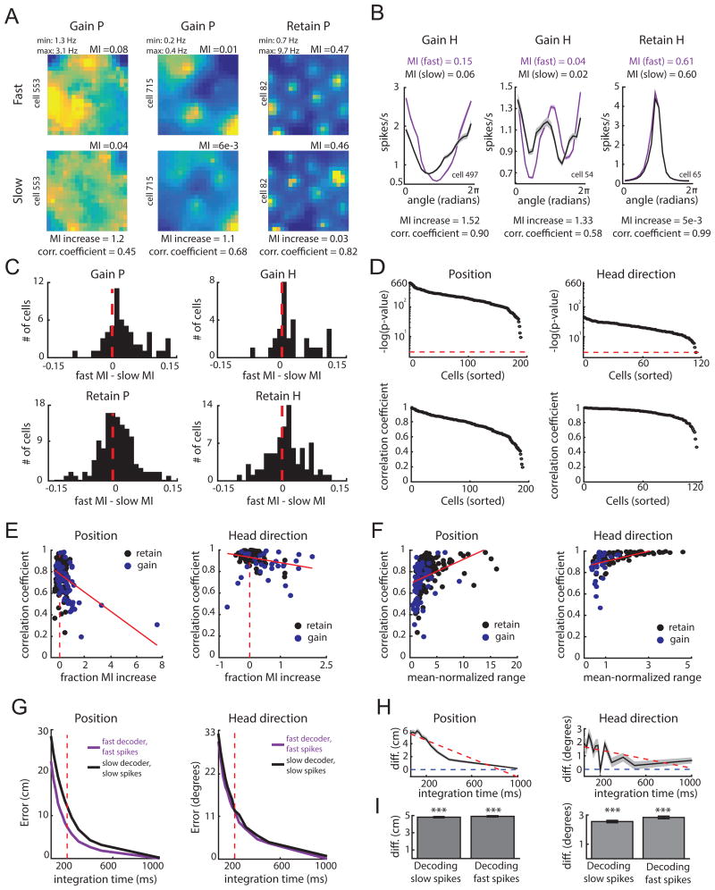
Figure 7.

Tuning is more informative at fast speeds and is adaptive. A-B. Example response profiles for cells that gain or maintain P or H coding (follows plot conventions of Figure 6). Response profiles, and all comparisons in this figure unless stated otherwise, are derived from the more complex selected model across epochs. For each pair, the mutual information (MI), fractional increase in MI [(MI_fast - MI_slow)/MI_slow], and Pearson correlation coefficients, are computed. C. Difference in MI for position (left) and head direction (right) for cells that gain P (top left) or gain H (top right) at fast speeds, and cells that retain P (bottom left) or retain H (bottom right) across speeds. D. Negative log of p-values (top) and coefficients (bottom) for correlations between the slow and fast-epoch response profiles for cells that gain or retained P or H coding. The red line indicates p = 0.05, with cells above this line attaining significance. E. Scatter plot of MI fractional increase and correlation coefficient between response profiles for cells that gained (blue) or retained (black) P (left) or H (right) coding features with fast speeds. Dashed red line indicates an MI increase of 0, while the solid red line indicates the best-fit line to the data. F. Scatter plot of the mean-normalized range of the slow-derived response profile and correlation coefficients from (E) for cells that gained or retained coding P (left) or H (right) with fast running speeds. G. Top: P and H decoding error of a decoder trained and tested on data derived from parameters of the selected model during fast epochs (purple) versus parameters of the selected model during slow epochs (black). H. Difference in error in decoding position (left) and head direction (right) between the slow and fast decoders in (G). I. Decoding error difference for position (left) or head direction (right) between the slow and fast decoder when decoding data from slow epochs (‘slow spikes’; left of each plot) or when decoding data from fast epochs (‘fast spikes’; right of each plot). Mean difference is computed by averaging across all decoding iterations and tested integration times. Error bars correspond to standard error of the mean across the decoding iterations. *** p < 0.001. (See also Figure S7)