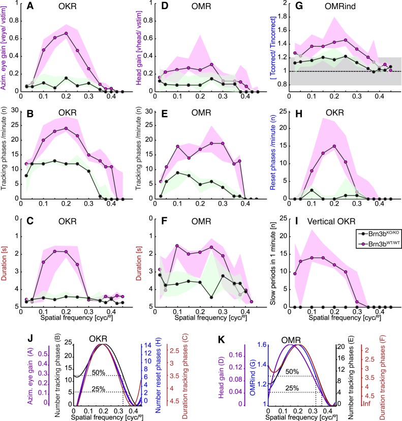
Fig. 4.

Comparison of OKR and OMR dependency on spatial frequency in Brn3b^KO/KO and Brn3b^WT/WT mice. A–F: spatial frequency dependency of gain (A and D), number (B and E), and duration (C and F) of tracking phases for OKR (A–C) and OMR recordings (D–F) of Brn3b^KO/KO (green; n = 3) and Brn3b^WT/WT mice (magenta; n = 3). Data are presented as medians (black lines) and observation ranges (shaded areas; observations represent medians of individual mice). For recording conditions and example traces, see Fig. 3. Note that the y-scale for C and F is inverted. G: automated OMR index for the same experiments as in D–F. Horizontal dashed line at 1 and shaded gray area (0.8–1.2) represent the OMR index median and interquartile interval for a blind mouse. H: number of reset phases for OKR experiments in A–C. I: vertical OKR recordings for Brn3b^KO/KO (green; n = 2) and Brn3b^WT/WT mice (magenta; n = 3). J and K: data for Brn3b^WT/WT mice shown in A–H were fitted following the fourth-order polynomial function (using the MATLAB curve fitting toolbox and the nonlinear least absolute residual method: f_(x) = a·x⁴ + b·x³ + c·x² + d·x + e. We used a degrees of freedom-adjusted R² value to determine the goodness of fit. For OKR measurements: number of slow OKR phases (black; data from B), R² = 0.84; number of reset phases (blue; data from H), R² = 0.68; gain (purple; data from A), R² = 0.80; duration of tracking phases (red; data from C), R² = 0.50. For OMR curves: number of tracking phases (black; data from E), R² = 0.80; OMR_ind (blue; data from G), R² = 0.72; gain of OMR (purple; data from G), R² = 0.46; duration of OMR phases (red; data from F), R² = 0.79. The curves were scaled for better comparison of the qualitative trends and are color-coded together with their respective axes.