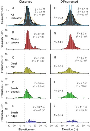
Fig. 2. Sample distributions of observed and corrected sea-level highstands.

(A) Distribution of the observed elevation data (4, 27, 28) after excluding outliers (8 of 298 data points) and accounting for spatial clustering of the data (see Materials and Methods). We capture the measurement uncertainty at each site by randomly sampling from the uncertainty range provided in each database. On average, we draw 10,000 samples per site. (B to E) Breakdown of the observed distribution by sea-level indicator type, as labeled (other indicators are not shown). (F to J) Observed distribution after correction for the set of four DT simulations that yield the highest correlation between predictions and observations (see fig. S8A). The mean ($\overline{x}$) and variance (s²) for each distribution are listed in each panel. We also indicate the correlation coefficient (R) between the data and the correction. The correlation in (F) is significant at a level of 90% (95%) if R > 0.16 (0.20). The correlations within the subsets in (G) to (J) are significant at a level of 90% (95%) if R > 0.21 (0.25), R > 0.26 (0.32), R > 0.22 (0.28), and R > 0.49 (0.59), respectively. The orange line in (A) and (F) indicates the best-fitting normal distribution, the cyan line shows a Student’s t distribution centered around the mean. Note that the variability among the different DT models follows a Student’s t distribution (see fig. S9). We used a kernel with 1-m bandwidth to calculate the maximum likelihood value ($\widehat{x}$; black line) listed in frames (A) and (F).