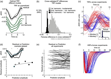
Fig. 2.

Optimal TRFs and HRFs. (a) Comparison of optimal TRFs for different models fitted to the same data set as in Fig. 1. Top “TRF as unpredicted residual” shows TRF estimated for the blank-subtracted fit, as the residual after regressing away all spiking-related components from the measured hemodynamics. Gray lines: individual contrasts; black: average across contrasts. The four traces below (green, in online version) show optimal TRFs from HRF+TRF fits, for models using progressively more Fourier terms from the fundamental alone up to the third harmonic; (traces are shifted vertically downward for visibility). Asterisk marks the fundamental + first harmonic, the same TRF as in Fig. 1(b3). Note the increasing high-frequency structure with increasing numbers of Fourier terms. (b) Using cross validation to test if increasing the number of TRF Fourier terms increases $R^2$ and improves the fit (1000 samples, 50–50 splits; each sample fitted with all four models). Histograms of pairwise differences in cross-validated $R^2$ for three pairs of models (see color coding; labels refer to the maximum number of harmonics in the Fourier series). We tested each pairwise difference of $R^2$ for an improvement in $R^2$ on adding more Fourier terms, against the null hypothesis that the two $R^2$ values are equal to each other (see Sec. 2.8). The $R^2$ for the fundamental + first harmonic was significantly higher than that for the fundamental alone ($p<0.017$ for the null hypothesis; see histogram for “first harmonic – fundamental”). However, there was no further improvement on adding the second ($p=0.44$) or the third harmonic ($p=0.30$; note that the corresponding histograms are largely centered on 0). Histogram bin size = 0.005. $Y$ Scale bar: $N=100$ counts for first harmonic – fundamental, and 600 counts for the other two. (c) Optimal TRFs across experiments (fundamental + first harmonic Fourier model), shown per monkey “S” ($N=40$) and “T” ($N=25$). Traces scaled by the amplitude (standard deviation) of the hemodynamic response for the experiment. Inset shows the histogram of the fitted optimal factors $P$ expressing the TRF Fourier fundamental period as a fraction of the trial period. The values are very close to 1 (median = 0.99 [0.95; 1.1], $N=65$, where the numbers in square brackets [..] mark the $-/+$ 34th percentile limits flanking the median, equivalent to $-/+1$ SD, Gaussian). (d): Top panel: residual unpredicted by spiking, same data set as Fig. 1, using the same optimal HRF. Same horizontal (time) and vertical scale as the TRF traces in (a). Color coded for stimulus contrast as in Fig. 1. Lower panel: amplitudes of the residuals, plotted against the amplitudes of predictions from spiking, color-coded for contrast. Amplitudes were quantified as the standard deviation over a trial, normalized to the prediction from spiking at the highest contrast. Line shows the linear regression. (e) Regressions between residual and spiking prediction calculated as in (d), shown for the full set of experiments. (f) Optimal HRFs, also separated by animal [same color coding as in (c)], shown normalized to the peak to help distinguish time courses. Note the distinct HRF time courses per monkey, consistent across experiments and recording sites (monkey S: $\tau =2.5$ [2.0 3.2]; $W=2.9$ [1.6 5.4]; monkey T: $\tau =5.6$ [3.1 8.0]; $W=4.0$ [2.7 6.0], where $\tau$: time to peak, $W$: peak full width at half maximum, and data are expressed as “median [min max]”).