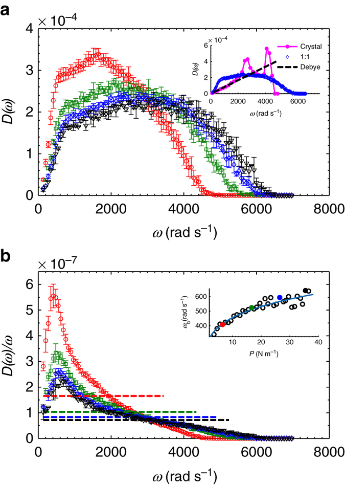
Fig. 2.

Density of states and the reduced density of states. a D(ω) for pressure (units N m⁻¹) P = 6.54 (red circles), 16.69 (green squares), 26.5 (blue diamonds) and 35.48 (black inverted triangles). Here each curve is ensemble averaged over 10 different runs at the same pressure. Inset: comparisons of D(ω) values of the disordered system at a pressure of P = 26.5 N m⁻¹ (blue diamonds) with those of the perfect hexagonal lattice (magenta) and Debye’s model (black dashed line). b The corresponding reduced density of states D(ω)/ω after normalizing the D(ω) in a with Debye’s scaling, i.e., ω in 2D. Dashed flat lines of the same color denote the corresponding Debye’s model, which is defined as $g_{\mathrm{D}}\left(\omega \right)∕\omega \mathrm{=}\frac{S}{4\pi N}\left(\frac{1}{v_{\mathrm{L}}^2}+\frac{1}{v_{\mathrm{T}}^2}\right)\mathrm{=}\frac{\rho S}{4\pi N}\left(\frac{1}{\left(B+G\right)}+\frac{1}{G}\right)$, where $v_{\mathrm{L}}\mathrm{=}\sqrt{\frac{B+G}{\rho }}$ is the longitudinal sound velocity, $v_{\mathrm{T}}\mathrm{=}\sqrt{\frac{G}{\rho }}$ is the transverse sound velocity, ρ is the mass density (mass per unit area), S is the area of the whole system, B is bulk modulus, G is shear modulus, and N is the total number of particles of the system. Inset: the BP frequency ω _b vs. the pressure P. Here the blue solid line is a power-law fitted curve, and the fitting function is ω _b = 271.5P ^0.224. The four filled circles of different colors represent the data points of the four curves of the matching colors shown in the main panel. Here all the error bars denote one SD around the mean value obtained from ∼10 realizations of each pressure