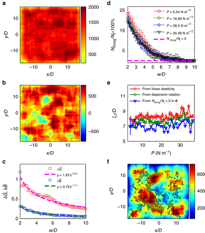
Fig. 6.

Heterogeneity of local moduli. Contour plot of the local bulk B a and shear G moduli b at P = 26.50 N m⁻¹. Here, the coarse-graining size w = 5D, where D is the mean diameter of the particles. Both B and G include affine and nonaffine components, and there are negative values in G but not in B. c Relative fluctuations of moduli $\delta \tilde{G}\equiv \frac{\delta G}{⟨G⟩}$ (red circles) and $\delta \tilde{B}\equiv \frac{\delta B}{⟨B⟩}$ (blue squares) that satisfy the power-law fitting (dashed lines). Here, $\delta \tilde{B}\propto w^{-1.11}$ and $\delta \tilde{G}\propto w^{-0.81}$. The data points here are ensemble averaged for seven realizations of P = 26.5 N m⁻¹,other pressures show the similar results, and the error bars are within the symbol size. d The percentage of the negative G vs. w at P = 6.54 (red circles), 16.69 (green squares), 26.5 (blue diamonds), and 35.48 (black inverted triangles) N m⁻¹. The characteristic length can be determined from the crossover between each curve and the zero line (i.e., the magenta dashed line). e Comparison of three characteristic lengths: (1) from linear elasticity values of $v_{\mathrm{T}}=\sqrt{G∕\rho }$ and ξ _T = 2πv _T/ω _b (red circles), (2) from the dispersion relation (green squares), and (3) from the above crossover (blue inverted triangles). The error bars in d–e signify one SD around the mean value obtained from ∼10 realizations of each pressure. f The spatial correlation between the nonaffine G (backgrounds) and the superposition of low frequency modes for ω < ω _b (black circles). Here, w = 7D