Figure 3.

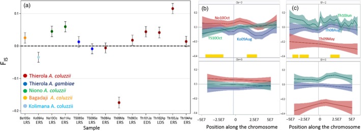
Departures from Hardy–Weinberg equilibrium measured by mean Fis (difference between observed and expected heterozygosity, expressed in units of expected heterozygosity) among samples and across the genome. (a) Least‐squares means of Fis and 95% CI computed in an ANOVA with locus (random effect) and population (fixed effects). Dotted horizontal line marks the expected value (zero). The seasonal acronyms under the x‐axis includes “RS” and “DS” to denote rainy and dry seasons, preceded by “E” or “L” to denote the early and late parts of each season, respectively. (b) Variation in Fis along the autosomes (chromosomes 2 and 3 in the top and bottom panels, respectively) in selected samples (note: colours alternate across plots). Nonparametric loess regression functions are used to detect trends and 95% CI (following Fig. S3)