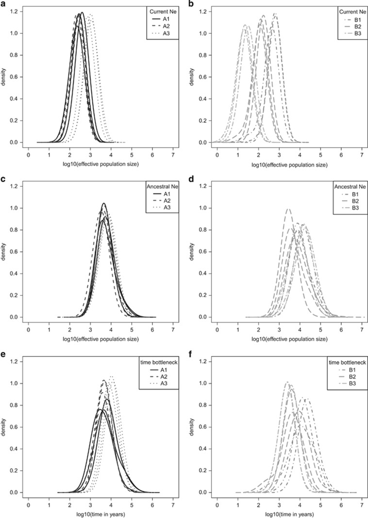
Figure 3.

Demographic analysis using MSVAR. For populations A1–A3 and B1–B3, their current effective population size is shown (a, b), the ancestral effective population size before the bottleneck (c, d) and the time of the bottleneck (e and f). The posterior distributions of each parameter for the A populations are shown in shades of dark gray, and for the B populations in shades of light gray. For each population, three distributions are shown for each parameter, as each population was analyzed using three alternative priors. The x axis is in log(10) scale, for example, 2 represents 100, and 4 represents 10 000.