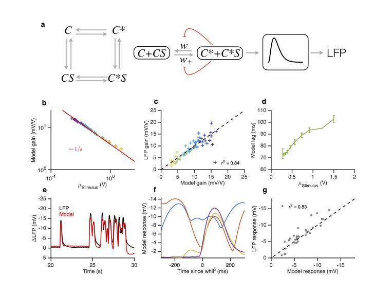
Figure 8. A modified two state receptor model reproduces Weber’s Law and adaptive slowdown in LFP responses.

(a). Or-Orco complexes (C) can be bound or unbound and active or inactive. (b) We assume (un)binding rates are much faster than (in)activation rates. Activity of the complex feeds back onto the free energy difference between active and inactive conformations, which also decreases the activation and inactivation rates of the complex (Equations 1–4). A mono-lobed filter converts receptor activity into LFP signals (Equation 5). We fit the model to Gaussian (Figures 3 and 5) and naturalistic data (Figures 1–2). In these fits, $\alpha =12.5 s^{-1}, \beta =1.26 s^{-1}, {\epsilon }_L=0.86, K_{on}=0.1 V$and $K_{off}=400 V$. (c) Model gain vs. mean stimulus. Red line is the Weber-Fechner prediction (${\displaystyle \mathrm{\Delta }R/\mathrm{\Delta }S\sim 1/S}$). (c) LFP gain vs. model gain. (e) Model response lag with respect to stimulus vs. mean stimulus. (f) LFP and model responses to naturalistic stimulus. (g) The model reproduces LFP responses to similar-sized whiffs that vary inversely with the size of preceding whiffs. (cf. Figure 2). (h) LFP responses vs. model responses for every whiff in the naturalistic stimulus.

DOI: http://dx.doi.org/10.7554/eLife.27670.021

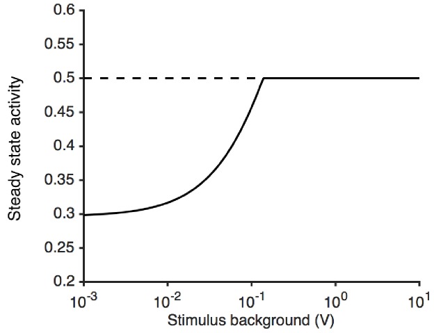
Figure 8—figure supplement 1. Steady state activity as a function of the stimulus background.

At high stimulus background, the steady state activity of the receptor complex is $a_0$ (here, 1/2). The model is unable to adapt perfectly to lower stimulus backgrounds, since $\epsilon$ is bounded by ${\epsilon }_L$. This causes the steady state activity to decrease.

DOI: http://dx.doi.org/10.7554/eLife.27670.022

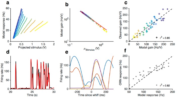
Figure 8—figure supplement 2. Front-end adaptation followed by a LN model reproduces firing rate responses to Gaussian and naturalistic stimuli.

(a–f) Model from stimulus to firing rate (see Materials and methods) fit to Gaussian and naturalistic stimuli. (a) Model responses vs. projected stimulus with increasing mean stimulus (cf. Figure 3). (b) Model gain vs. mean stimulus. Red line is the Weber-Fechner prediction (${\displaystyle \mathrm{\Delta }R/\mathrm{\Delta }S\sim 1/S}$). (c) Firing rate gain vs. model gain. (d) Firing rate and model responses to naturalistic stimulus. (e) The model reproduces variation in the firing rate responses to similar-sized whiffs (cf. Figure 2). (f) Firing rate responses vs. model responses for every whiff in the naturalistic stimulus.

DOI: http://dx.doi.org/10.7554/eLife.27670.023