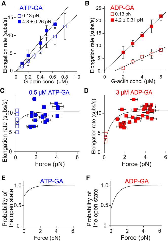
Figure 3.
Force-dependence of actin polymerization in the absence of profilin. (A and B) Given here are elongation rates under various ATP-G-actin (A) and ADP-G-actin (B) concentrations. Open and solid symbols represent mean elongation rates in low-tension single- and high-tension double-trap experiments, respectively. The numbers of actin dumbbells examined were as follows: 3, 4, 20, 6, 10, 6, 9, and 9 (single-trap) and 3, 11, 4, 4, and 3 (double-trap) from lower to higher ATP-G-actin concentration; and 5, 5, 6, 6, and 5 (single-trap) and 5, 14, 4, 3, and 5 (double-trap) from lower to higher ADP-G-actin concentration. Low and high-tension plots were globally fitted with Eq. 1 using corresponding tensile forces: 0.13 pN for low-tension experiments (estimated from the viscous drag), and the mean tensile forces 4.3 (ATP-G-actin) or 4.2 pN (ADP-G-actin) for high tension experiments (measured from the avidin bead displacement). Note that the curve with Eq. 2′ is identical to that of Eq. 1 because these two equations are essentially the same, except that the p0c in Eq. 1 is replaced with p0depoly in Eq. 2′. Error bars indicate mean ± SD. The optimal fitting curve values are shown in Table 1. (C and D) Given here is the force dependence of the elongation rate at specific G-actin concentrations: 0.5 μM ATP-G-actin (C) and 3 μM ADP-G-actin (D). Double-trap experiments (solid symbols) were performed at various tensile force ranges (including other than 3.5–5.5 pN). Each plot is from individual actin dumbbells. Parts of these data (3.5–5.5 pN) are included in the plots of (A) and (B). Single-trap experimental data (open symbols) are also shown. Computed curves are shown, constructed by Eq. 1 with values obtained by fitting in (A) and (B); (Table 1). Horizontal error bars indicate mean ± SD of the tensile force during measurement. (E and F) Given here is the force dependence of the open state probability. The open state probability in the stair-stepping model, described as 1 – p0cexp(−fd/kBT), was computed using the values obtained by fitting in (A) and (B) (Table 1). To see this figure in color, go online.

