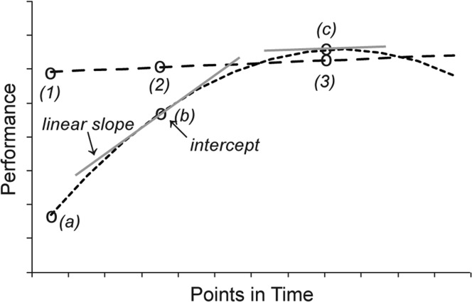
Figure 1.

Examples of two theoretical HLM curves are shown (dotted and dashed lines) with the components indicated. Intercept is the expected performance at a point in time (the centering point) on the basis of the HLM analysis of the group data. Three example intercepts are indicated with open circles along each curve (1, 2, and 3 along the dashed line and a, b, and c along the dotted line). Expected performance at the earliest point is much higher along the dashed line (1) than the dotted line (a). Linear slope is the rate of change at a specific point in time (the centering point)—that is, the slope of the tangent (gray lines) to the curve at the given time point. The linear slope at the intercept (b) is considerably steeper than the linear slope at the intercept (c). The rate of change is greater at the earlier time point. Curvilinearity is change in the linear component over time. The two example HLM curves differ in curvilinearity. The change over time is minimal for the dashed line and substantial for the dotted line. Each component and each condition has its own significance test that indicates if the parameter estimate is different from 0. For example, it is likely that the linear slope at (b) in Figure 1 would differ from 0, but the linear slope at (c) would not differ from 0. Comparisons of the components between CI conditions were conducted using chi-square tests.

Figure from Reeder, Firszt, Holden, and Strube (2014, p. 1113). Reprinted with permission.