Fig. 5.

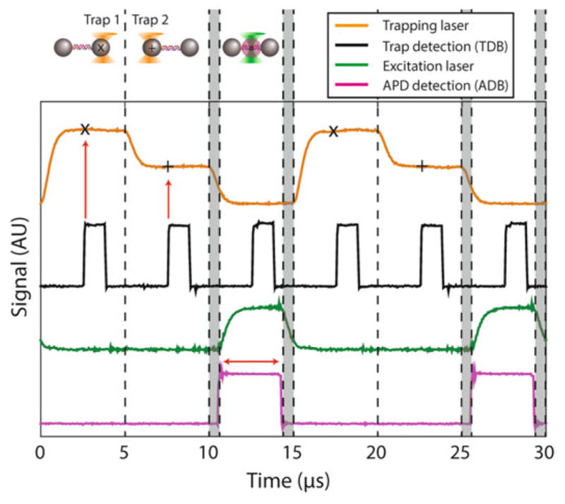
Interlacing and timesharing of optical trap and fluorescence excitation lasers, and synchronization of lasers with data acquisition timing. Two optical traps (orange) are created in sequence during two thirds of the interlacing period by time-sharing. The trap AOM (AOM1) switches between two deflection angles (traps in each interval are set to different intensities for clarity in the figure). Trap data acquisition occurs at time points centered on each trap interval. “×” and “+” denote the time points for the first and second trap, respectively. The rising edge of a digital pulse (black) is synchronous with the trap data acquisition timing (red vertical arrows). The fluorescence excitation (green) is only ON during the last third of the interlacing period while the trap is OFF. There are 625-ns delays (grey shaded regions) between turning OFF (ON) the optical traps and turning ON (OFF) the fluorescence excitation. A digital pulse (magenta) synchronous with the APD data acquisition timing is centered on the excitation laser interval. Fluorescence emission signals are only collected during this third time interval (red horizontal arrow). Laser intensities in the plot are measured by feedback photodetectors QPD1 and PD (see Fig. 3), and digital pulses synchronous with data acquisition timing are output directly from the DAQ card trap input timing debug (TDB) and APD gate timing debug (ADB) lines (see Fig. 10). All are recorded using a digital oscilloscope