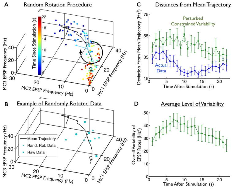
Fig. 4. Perturbed constrained variability.

(A) We constructed surrogate data in which the mean trajectories evoked by each stimulus (black solid curve; data shown are for one stimulus), and the overall levels of trial-to-trial variability, matched the recorded data, but the variability was distributed relatively isotropically over the space of neural responses. To do this, we took the constellations of points recorded at each epoch, and rotated them in a random direction about the mean response recorded at that epoch; this is shown schematically for the teal data points, corresponding to responses recorded 8s post-stimulation. (B) The raw data points observed 8s post-stimulation (teal circles) are shown alongside an example of the randomly-rotated data points (stars) from that same epoch. (C) For these perturbed surrogate data, we computed the distance from each response to the mean response trajectory associated with the applied stimulus. We then averaged these over all stimuli and experiments, and show those distances as a function of time post-stimulation (green curve). This is similar to the measurement shown schematically in Fig. 3A. For comparison, we also show the same quantity for the actual experimental data, in which the structure of the fluctuations was left intact (blue curve; same data as in Fig. 3C). (D). As in Fig. 3E, we measured the average trial-to-trial variability in the surrogate responses (with perturbed trial-to-trial variability) as a function of time. By construction, this level of variability is identical to that which was displayed by the actual (unperturbed) responses (in Fig. 3E). Error bars in all panels represent the standard error of the mean (S.E.M.) over all 4 stimuli and 9 slice experiments.