

Abstract
Various topics taken from the author’s research portfolio that involve multicomponent alloy solidification are reviewed. Topics include: ternary eutectic solidification and Scheil-Gulliver paths in ternary systems. A case study of the solidification of commercial 2219 aluminum alloy is described. Also described are modifications of the Scheil-Gulliver analysis to treat dendrite tip kinetics and solid diffusion for multicomponent alloys.
Introduction
For the Hume-Rothery lecture at the The Metals Materials and Minerals Society (TMS) meeting in Orlando on March 16, 2015, I decided to describe some of my work on solidification of multi-component systems. It is important to include efforts to treat multicomponent systems in the education of students and in fundamental research as we transition our science knowledge to engineering design of alloys. The fact that more than one composition variable must be tracked during solidification and solid state phase transformation leads to a path in composition space that adds complexity and richness to materials science not present for binary alloys. Analysis of these problems is closely related to phase diagrams.
William Hume-Rothery started his career doing very traditional phase diagram measurements in the 1930’s [1]. He pioneered the use of powder diffraction and extraction of intermetallic compounds from complex microstructures for chemical analysis before microprobe analysis was available. His desire to synthesize the knowledge gained from many alloys systems led him naturally to the work with which most of us are more familiar, the beginnings of the theory of alloy phases.
The education and research guidance given to me by my professor at the Johns Hopkins University, Robert Barrett Pond, is greatly appreciated. He was well known for giving lectures to American Society for Metals (ASM) chapters entitled, “Fun with Metals” [2] and for early patents of melt spinning techniques [3]. He taught ternary systems with models made out of plaster that showed the various single, two-phase and three phase volumes of a simple ternary eutectic system. Without this early exposure to ternary systems, I likely would have avoided multicomponent systems during my career.
Practical alloys typically contain many components and a discussion of solidification in ternary alloys is appropriate and the study of ternary phase diagrams is essential. For most casting situations the concept of local equilibrium at the liquid–solid interface(s) is applicable. The concept is based on the fact that the liquid-solid interfacial region relaxes to equilibrium much faster than over the larger microstructural scale. Thus the phase diagram is essential as it gives the possible interface conditions during solidification.
For ternary and higher order systems, extra information regarding tie-lines to specify equilibrium relations between phases is required. Tie-lines are trivial in binary systems. Tie-lines are isothermal lines that connect the compositions of the two phases in two phase regions of the phase diagram, for example for the liquid and solid. The concept of the tie-line in ternary alloys is easily employed in non-graphical methods to treat phase equilibrium in higher order systems. For solidification of a single solid phase from a ternary liquid, the tie lines can be described by a pair of partition coefficients, for the relationship between the solid and liquid composition for each alloying addition at the interface. The superscript E is used to indicate an equilibrium value and the asterisk is employed to emphasize that the values are interface quantities. In general the are not constants and depend on temperature and/or composition themselves. For multicomponent alloys the use of a Calphad-type approach [4] to efficiently deliver tie-line data is essential. I omit in this paper situations where a loss of interfacial equilibrium occurs and the partition coefficients become functions of interface velocity.
Many texts are available for the study of ternary phase diagrams [5–8]. One difficulty with these standard texts is that discussions of solidification always assume global equilibrium during cooling rather than local equilibrium. The greatest value comes from learning the structure of the phase diagrams considering global equilibrium, but then using them to describe conditions of local interface equilibrium. These conditions are inserted into models of solidification that treat the transport of the alloying additions via liquid diffusion, solid diffusion and fluid flow.
This paper will describe a model of ternary eutectic solidification and Scheil-Gulliver paths in example ternary systems. A case study of the solidification of commercial 2219 aluminum alloy used for early models of the Space Shuttle external tank will be described. Also described are modifications of the Scheil-Gulliver analysis to treat dendrite tip kinetics and solid diffusion for multicomponent alloys.
Ternary Eutectic
My PhD thesis in 1972 [9] involved the direct observation of the solidification of the Sn-Pb-Cd ternary eutectic chosen due to its low melting temperature of 145 C [10]. The microstructure is shown in Figs. 1 and 2. There are three lamellae with stacking αβγβαβγβα where α is the Sn-rich phase, β is the Pb-rich phase and γ is the Cd-rich phase. The thesis focused on how changes in the solidification rate affect the changes in eutectic spacing. In the thesis I also extended the Jackson and Hunt eutectic model of 1966 [11] to a ternary eutectic, which I now describe.
Figure 1.
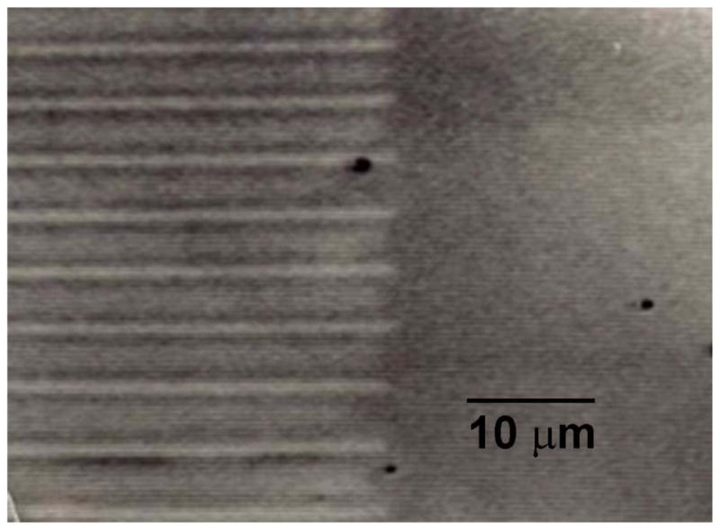
Microscopic in-situ observation of directional solidification of Pb-Sn-Cd ternary eutectic using moving temperature gradient hot stage. The bright phase is Cd, which is coated on both sides by the barely visible dark Pb phase. The gray is the Sn phase. The sample is held in a glass cell and the contrast is due to cross polarized light.
Figure 2.

Optical micrograph of etched Pb-Sn-Cd ternary eutectic. Sn is white, Pb is gray and Cd is black. Nital etch.
Consider the composition distribution in front of a triple lamellar interface that develops due to liquid diffusion. The interface will be assumed planar for the diffusion analysis. The coordinate system is chosen to be fixed on the flat interface which is growing edgewise into the liquid at a constant velocity V. The coordinate system, order of stacking and the notation for lamellar widths are shown in Fig. 3. The lamellar spacing is given by λ = 2Sα + 4Sβ + 2Sγwhere the S values are the lamellar half widths.
Figure 3.

Schematic of triple stacking of the lamella: α is Sn, β is Pb and γ is Cd. The lamellar spacing is defined as the distance between the centers of adjacent α phase lamellae.
With x and z defined in Figure 3 and assuming the off-diagonal liquid diffusion coefficients are zero, the linear constant coefficient diffusion equations for steady solidification for each solute profile in the liquid CLi (x, z) are
| (1) |
Due to periodicity, a solution CLi (x, z) needs to be sought only in the region z ≥ 0, 0 ≤ × ≤ Sα + 2Sβ + Sγ. The boundary conditions are
| (2) |
At x = 0 and x = Sα + 2Sβ + Sγfor all z
| (3) |
At z = 0 and 0 ≤ x ≤ Sα.
| (4) |
and at z = 0 and Sα ≤ x ≤ Sα + 2Sβ
| (5) |
And at z = 0 and Sα + 2Sβ ≤ x ≤ Sα + 2Sβ + Sγ.
| (6) |
where and are the ternary eutectic liquid, α, β, and γ phase compositions respectively.
Here the approximation has been made that and so on for the other solid phases. This assumption is consistent with that made by Jackson and Hunt. It means simply that compared to the solid phase compositions, the liquid compositions in front of each growing phase at the interface are close to the eutectic compositions.
The solution is
| (7) |
where
| (8) |
Here the assumption has been made. This assumption is again consistent with the Jackson & Hunt theory. The quantity, , is zero if the molar volumes of the phases are equal and if the liquid far from the interface is of eutectic composition. For the purpose of this paper it is interesting merely to point out the richness of the ternary eutectic case compared to the binary. Fig. 4a shows the liquid composition computed from Eqns.7–8 as one traverses the liquid-solid interface using the parameter values:
Figure 4.

Calculated composition at the liquid-solid interface for Pb-Sn-Cd ternary eutectic. a) profile across interface, b) same data plotted as a path superimposed on ternary liquidus projection.
For example, in front of a Sn lamella, Sn is being consumed by the growing lamella so its composition is low. But the Sn lamella is rejecting the Pb and Cd into the melt. Thus the Pb and Cd levels are high in front of the Sn lamella. The path of compositions across the interface is indicated by the lower case letters and is plotted on the ternary triangle in Fig. 4b. It is interesting that the path avoids the Pb-rich side of the eutectic composition.
The assumption of local interface equilibrium for the ternary eutectic solidification model requires that the liquidus surfaces for each of the three solid phases be extrapolated below the eutectic temperature in order to accommodate the calculated liquid compositions at the interface in front of each phase. As shown in Fig. 5, the three extrapolated liquidus surfaces form the three faces of a triangular pyramid formed when they are intersected by an isothermal plane below the eutectic temperature. The vertex of the pyramid is the eutectic point and the edges of the pyramid, which intersect at the vertex, are the extrapolated lines of the three monovariant binary eutectics.
Figure 5.

Schematic drawing of the three extrapolated liquidus surfaces below the ternary eutectic temperate (triangular pyramid) showing the variation of the constitutional undercooling, ΔTC, and the capillary undercooling, ΔTσ, as one traverses the lamellar interface. The sum of the two is the total eutectic interface undercooling.
Based on the local liquid compositions across the interface, the local temperatures across the interface would follow the serpentine curve lying on the surface of the triangular pyramid in Fig. 5. This is the constitutional (compositional) part of the undercooling below the thermodynamic eutectic temperature at each location on the liquid solid-interface. Because the lamellar interface is practically isothermal (at the base of the pyramid), the remainder of the variation in undercooling across the interface is made up of the undercooling due to variation of curvature of the individual lamella according to the local Gibbs-Thomson effect.
The theory was completed by computing the average composition in front of each lamella and the average curvature of each lamella, to yield an expression for the total undercooling as a function of λ and v. Employing the extremum condition (spacing that produces minimum total undercooling for given velocity) then yields the standard expression, λ2V = constant.
More recent work extending the Jackson-Hunt analysis to a variety of ternary eutectic structures has been published by Himemiya and Umeda [12]. Phase field models are being used to investigate the solidification of ternary eutectics [13]. For a binary eutectic to which a small amount of a third element is added, a Mullins and Sekerka type instability of the binary eutectic front occurs and eutectic colonies form. Phase field simulations of colony formation have been performed by Plapp and Karma, [14] as shown in Fig. 6. If a larger amount of a ternary element is added to an alloy lying on a monovariant eutectic valley, a eutectic colony can actually evolve into a two-phase dendrite with secondary arms [15]. Between the two-phase dendrite, ternary eutectic is found. Fig. 7 shows a micrograph of a quenched liquid solid interface of such a growth form in Pb-Sn-Cd system [16]. Spiral two phase dendrites have recently been observed by Akamatsu et al. [17] and modeled by Rátkai et al. [18]. A parabolic shape composed of the two solid phases forms a double helix. This growth mechanism permits the eutectic spacing to maintain a near constant value for a specified growth rate.
Figure 6.

Phase field simulation of monovariant binary eutectic in a ternary system showing the development of the colony structure (Plapp and Karma, 2002). The long range diffusion of solute ahead of the eutectic front as well as the shorter range diffusion on the lamellar scale is apparent.
Figure 7.

Quenched interface of a two phase dendrite of Sn-rich and Cd-rich phase growing ahead of the ternary eutectic interface. The alloy composition lies on the monovariant eutectic valley, L → Sn + Cd in the ternary system Sn-Pb-Cd.
Scheil-Gulliver Solidification
Use of the Scheil-Gulliver approach to determine the solidification path is quite useful for practical casting modelling where solidification usually occurs by a dendritic mechanism. This became clear to the author during a NIST sponsored Consortium on Casting of Aerospace Alloys between 1992 and 1998 involving industry and university researchers. It was determined that a simple Scheil-Gulliver model employing thermodynamic databases for practical alloys could deliver good estimates of the enthalpy vs. temperature data over the alloy freezing range. Indeed incorporation of such a tool within commercial heat flow casting software used by casting engineers to determine the best locations of sprues, risers and chills was needed.
Scheil-Gulliver analysis of solidification is possible and widely available within thermodynamic phase equilibria codes because of the extremely simplifying assumptions that require no diffusion analysis. A volume is chosen within a casting in which the temperature can be treated as uniform but decreasing. The liquid within this volume is assumed to be well-mixed and solid diffusion is forbidden. There are no nucleation barriers. If one is only interested in how conditions change with fraction of solid, no assumption regarding the shape of the liquid-solid interface is necessary. For example, the solid composition as a function of fraction solid (microsegregation or coring pattern) is readily predicted. However predicting the solid composition as a function of distance as might be measured with a microprobe within an interdendritic region requires geometrical assumptions regarding the growth morphology; e.g., cylindrical or spherical dendrites. As described below, Scheil-Gulliver models can be “patched up” to treat situations where the assumptions are violated. Best results would come from 3-D phase field models that incorporate thermodynamic parameters from Calphad type databases. This is an active area of research [19, 20], but a simpler approach as described here remains useful.
A schematic comparison of the Scheil-Gulliver solidification of alloys with three different ternary phase diagrams is shown in Fig. 8. In the three ternary systems considered, the α, β, and γ phases are solid solutions based on pure A, B, and C respectively. The δ phase is an intermetallic based in the A–B system. In Fig. 8b, the intermetallic forms from the melt congruently, whereas in Fig. 8c, it forms by a peritectic reaction.
Figure 8.


Schematic of the interface shape and microstructure produced during dendritic solidification of three ternary alloys with different phase diagrams, a), b), c). The dotted rectangle shows the “Scheil box” at two different temperatures. See text for details.
The figure shows the liquidus surfaces and schematic microstructures. In the latter, the solid is considered to grow in a vertical temperature gradient. Because heat is transported so much faster than solute, it is appropriate to think of temperature as decreasing from the top to the bottom with no lateral gradients. The volume considered for the Scheil-Gulliver approach is shown dashed and can be thought of as a box, hereafter termed the “Scheil box,” moving down through the microstructure as the solidification occurs and the temperature drops. Conversely, the microstructure can be thought of as moving upward through the box. Within the Scheil box the liquid composition is uniform at each height (temperature), but changes with temperature (vertical position). A plot of this changing liquid composition superimposed on a liquidus projection of the phase diagram is called the solidification path. The solid develops a composition gradient as solidification proceeds.
Solidification starts at the liquidus temperature. The first phase to form is the α phase in all cases and is depicted as a large cell in the microstructure sketch even though it might be dendritic with side branches in reality. As the solidification continues, the box moves downward as the entire liquid portion of the box becomes enriched in component B and C following the liquidus surface. If the α solid solution were pure A (zero partition coefficients), the liquid composition would follow a linear path directly away from the A corner of the phase diagram. If the α solid solution contains solute elements (nonzero partition coefficients), the prediction of the Scheil-Gulliver approach induces curvature in the path. Only the increment of α phase solid forming at each instant follows the solidus surface (not shown) leaving behind a microsegregated solid. As the fraction of solid increases (the box moves down further), the liquid composition and the temperature approach the monovariant lines on the liquidus surface of the phase diagrams, T2 in (a) and T1 in (b).
For cases (a) and (b) the monovariant lines are of eutectic character and constitute valleys on their respective liquidus surfaces. However unlike a eutectic in a binary system, this eutectic forms over a range of temperature and the remaining liquid in the box follows the valley as temperature decreases. The solid forming during this process is a two-phase mixture composed of α + β (Fig. 8a) or α + δ (Fig. 8b) as show schematically. The phase compositions as well as the phase fraction of the eutectic remaining in the solid microstructure will in general vary as the remaining liquid descends the liquidus valley. The case where the liquid path crosses a peritectic monovariant line is shown Fig. 8c at T1. Here, solidification switches from α to δ phase; i.e., α stops forming and δ begins and continues solidification as a coating on the α phase.
In Fig. 8a the liquid at lower temperature finally reaches the ternary eutectic composition and forms a three phase microstructure at a single temperature TE with a planar L–S interface as L → α + β + γ. In Fig. 8b, the liquid encounters a special point at T2 where two eutectic valleys meet to form a third that continues down in temperature. This point represents the liquid composition of the invariant reaction, L + α → δ + γ. When the liquid reaches this point on the phase diagram, the solidification switches from leaving a two phase coating of α + δ on the original α dendrite to leaving an additional coating of a different two phase eutectic of δ + γ. Solidification of this alloy is finally completed at a ternary eutectic point TE where β, δ, and γ phases form at a single temperature (planar liquid–solid interface). For the case of Fig. 8c, the path traverses the δ liquidus surface, between temperatures T1 and T3 until it intersects the monovariant eutectic valley L → δ + γ at T3. The path then follows this valley forming a two phase mixture of δ + γ until the freezing is completed at the ternary eutectic temperature TE.
This is an idealized description even beyond that imposed by the Scheil-Gulliver approach. The drawings assume that the various eutectic solidification processes all form fine multiphase structures accomplished by coupled growth. In particular cases, the phases may form irregular or divorced eutectics if one or more phases are facetted or if the space remaining between the dendrites is small compared with the spacing of the eutectic. Then the phases may form in the interdendritic regions in an uncoupled eutectic fashion.
Quantification of the solidification path for an n-component alloy describes the composition of liquid and solid as a function of fraction solid fS. These functions are intrinsically different. The first represents the composition of not only the interface value but also the entire liquid within the Scheil box at each value of fraction solid (temperature). The latter represents the composition of the solid forming at that value of fraction solid but also the solid composition profile that is “frozen-in” characterizing the coring pattern within solidified structure.
Using conservation of solute, the liquid composition is obtained from the set of n − 1 equations during primary solidification as
| (9) |
which are uncoupled if the partition coefficients, , do not depend on the composition of the other species. If the are constants, integration leads to
| (10a) |
for an alloy of initial composition C0i. The interface temperature at this value of the fraction solid is given by
| (10b) |
if the liquidus slopes, , can be treated as constants. For a ternary alloy, a plot of vs. superimposed on the liquidus projection of the phase diagram shows the solidification path for the primary phase.
Beyond primary solidification, one then determines the fraction solid at which the liquid composition crosses a monovariant eutectic line and where an additional solid phase begins to form. The liquid path then follows this line because deviating from this line in either direction causes an increased formation of the corresponding solid phase. This process returns the liquid composition back to the eutectic line.
If the liquid path encounters a monovariant peritectic line, different considerations are necessary. Because of the Scheil-Gulliver assumption of no solid diffusion, the peritectic reaction as normally described in text books does not occur. The solidification path for the liquid does not follow the line of peritectic reaction because any deviation from the line does not produce a return to the line as for the eutectic case. The path merely crosses the line with a corresponding change in the solid phase being formed.
Scheil-Gulliver analysis is performed within thermodynamic codes by stepping down in temperature. Rewriting Eqn. 9 and changing to finite differences, one obtains
| (12) |
which provides the basis for the following stepping procedure. An equilibrium calculation is performed for the initial (liquid) composition at a temperature just below the liquidus temperature in the two phase liquid plus solid region. The tie-line in this two phase region gives the composition of the liquid and solid as well as the lever law phase fraction of solid that is equal to the quantity . This lever law fraction of solid is the first incremental change of solid fraction from zero. The temperature, liquid and solid compositions and fraction solid are stored. This process is repeated at the next lower temperature step using the liquid composition obtained in the previous step as the new average composition for the tie-line determination. Again the liquid and solid composition is stored and the lever law fraction of solid multiplied by the remaining liquid fraction (1 − fS) is incrementally added to that from the previous step. An important consideration is that the temperature step be small as one is approximating the solution to a differential equation.
If the individual equilibrium calculation reveals that the liquid has developed equilibrium with two solid phases, the compositions of the two solid phases are stored and their increments accumulated as before. This would be the case when a eutectic line is encountered. If a peritectic line is encountered, the stepping procedure would naturally reveal that a different solid phase would form and its solidification would be tracked.
Enthalpies of the system can be computed at each temperature based on the phase fractions and the average phase compositions. The average composition of each solid phase can be computed at each temperature by numerical integration of the compositions vs. phase fraction information obtained during the Scheil-Gulliver calculation. (See eqn. [20] below.) Summation of the individual phase enthalpies times their accumulated phase fractions is employed to compute the total enthalpy at each temperature. Rather than using the average solid phase composition, one may perform an integration of the enthalpy of each increment of solid phase fraction that has different compositions. However it has been shown that the use of average phase composition in the computation of the enthalpy is a good approximation [21]. This enthalpy calculation is of major importance to the casting engineer assigned the task of modelling the heat flow.
Space Shuttle Tank Alloy Study
Early in my career, in 1977, the Metallurgy Division of the National Bureau of Standards, or NBS (now NIST) was asked to evaluate the 2219 aluminum alloy plate used in the fabrication of early versions of the external fuel tank for the space shuttle [22–23]. In 1977 no launches had yet occurred. Soft spots had been discovered in 2024 aluminum plates, due to improper quench from solution heat treatment temperature. Although no soft spots were discovered in 2219 produced at the same plant, NASA asked us to determine how much 2219 would have suffered if the same improper heat treatment had occurred during its processing. Most of the work had to do with the establishment of C-curves (TTT) for the properties for the slack quench from solution heat treatment temperature but with normal stretch and aging for 2219. We employed heat flow calculations of the slack quench combined with the measured property C-curves to determine the yield strength for plates of different thickness for worse case quench conditions. It was determined the specifications for the alloy were met as long as the plate was thinner than 5 cm.
The technical leader of the project was Robert Mehrabian, chief of the Metallurgy Division. Because of his interest in solidification, I was asked to evaluate the macro- and microsegregation in the Direct Chill (DC) semi-continuous cast 2219 ingots, which nominally contained about 6.3% Cu (mass fraction). Typical macrosegregation of copper in one of these ingots is shown in Fig. 9. The chill face composition is 18 % Cu. This region is removed by scalping prior to further processing. Near the centerline the composition drops to 5.5% Cu. The variation of the other elements was not measured. The segregation typically remains in plate products after rolling.
Figure 9.

Macrosegregation profile, average copper content vs. distance from the chill face, across the short transverse x-direction (inset) of a semi-continuous DC cast ingot of 2219 aluminum alloy. The variation of the other alloying additions was not measured.
In order to determine the effect of composition on properties, a quick study was conducted with a special directional casting geometry with a cross section area change [24]. Fig. 10 shows the casting geometry and the macrosegregation produced in the vertical direction. A dip in Cu content occurs in the vicinity of the cross-section change. From this casting slices were cut at different heights, each having a different composition. These samples were rolled and heat treated normally to T87 temper to determine how the properties varied with composition. As shown using the right axis of Fig. 10, the properties were acceptable as long as the composition remained above 5.5% Cu. Because the lowest copper content observed in the center of the DC ingot was ≈5.7% Cu (Fig, 9), the macrosegregaton in the 2219 ingots was not believed to cause degradation in mechanical properties.
Figure 10.

Variation of average Cu content % mass fraction vs. distance (solid line) from the chill face of a specially designed unidirectionally solidified cross-section change casting (see inset) of 2219 Al alloy. Horizontal slabs taken from the casting were roll-reduced 10:1 and heat treated to the T87 condition. The dashed line shows the hardness of these samples after heat treatment.
The microsegregation was also examined. The 2219 alloy material analyzed had a composition of Al-6.63% Cu, −0.3% Mn, −0.2% Fe −0.1% Si (mass fraction). Fig. 11 shows the globular dendritic microstructure of the aluminum primary phase. Between the dendrites are needles of βAl7Cu2Fe and a fine two phase mixture of aluminum and Al2Cu. At the time, no Calphad type calculations were available. I wanted to see if I could predict these phases using existing phase diagrams and a Scheil Gulliver method. To employ existing ternary liquidus data, an effective ternary composition was required. The amount of Mn was added to that of the Fe, the Si was ignored and the ternary system Al-Fe-Cu ternary liquidus projection of Philips [25] was employed. A Scheil-Gulliver solidification path for the aluminum primary phase was computed using constant binary partition coefficients taken from the binaries of kCu=0.17 and kFe=0.02. The path is superimposed on the liquidus surface in Fig 12. The solidification path traverses the aluminum liquidus surface, hits eutectic valley for L → Al + βAl7Cu2Fe thereby forming the βAl7Cu2Fe phase along with the aluminum phase, and finishes solidification with the ternary eutectic, L → Al + βAl7Cu2Fe + Al2Cu. This predicted sequence of phase is identical to that observed experimentally as shown in Fig. 11. Note that the needles of βAl7Cu2Fe are not finely intermingled with the fine αAl + Al2Cu structure and they form an uncoupled eutectic due to their facetted nature.
Figure 11.

a) Micrograph od dendritic structure of as-cast 2219 Aluminum alloy. b) Micrograph of interdendritic region. The ends of the needles of Al7Cu2Fe are imbedded in Al dendritic matrix showing that the needles formed along with the Al as a divorced (uncoupled) eutectic L → Al + Al7Cu2Fe. Later freezing and shows a fine two phase mixture of Al + Al2Cu with additional needle-shaped Al7Cu2Fe for the ternary eutectic, L → Al + Al7Cu2Fe + Al2Cu.
Figure 12.

By adding the Fe and Mn contents for the 2219 alloy and ignoring the Si content, a Scheil-Gulliver path can be calculated using partition coefficients obtained from the binary Al-Fe and Al-Cu binary diagrams. After the freezing of the Al phase, the path intersects the L → Al + β eutectic valley before reaching the ternary eutectic, L → Al + β + CuAl2. The α phase is Al6Fe and the β phase is Al7Cu2Fe.
To analyze the situation further in 1977 prior to the availability of Calphad thermodynamic engines and databases, I resorted to a paper from 1950 by Phragmen [26], that I had studied as a graduate student. He measured phase diagrams for the Al-rich portion of the 6 component system Al-Cu-Mn-Mg-Fe-Si. I had been required to study this paper as a student under Professor Pond. Phragmen produced quaternary tetrahedrons of the liquidus projection using the ternary liquidus projection as its faces and filled in the internal phase space of the tetrahedron by experimental measurements. To graphically display the quaternary data in a 2-D figure, he projected the multivariant eutectic and peritectic lines involving the aluminum phase within the tetrahedron away from the aluminum corner and onto the opposite face of the tetrahedron. This produced a triangular diagram with composition axes in relative amounts of the other elements omitting Al. These diagrams can only be used if the Al phase is the first to form.
A portion of such a plot is shown in Fig. 13 for the Al-Fe-Cu-Si system. If the entire triangle were shown, the corners of this triangle plot would be CuAl2, FeAl3 and Si. For the alloy 2219 alloy of interest here, the relative mass fractions are 91.6% Cu, 4.2% Mn, 2.8% Fe and 1.4% Si. Again adding the Fe and Mn contents, we plot the relative mass fractions 91.6% Cu, 7.0% Fe and 1.4 t% Si. This is point (a), which is located in the region labelled (Al,Cu)6(Fe,Cu). This phase is often called just Al6Mn with which it is isomorphous. Solidification starts with formation of the Al phase, which hardly changes the relative composition of the liquid in this diagram because mostly the Al component is being solidified. The location of point (a) means that after primary aluminum is finished, solidification would continue as L → Al + (Al, Cu)6 (Fe, Cu). Because the liquid is being depleted in mostly Fe through this process, the path for the liquid composition would move in a direction away from the Fe corner as shown. The path then intersects the boundary with the Al7Cu2Fe region in the diagram at point (b). Phragmen indicated the line to be of peritectic character and thus the path crosses over it and begins solidification L → Al + Al7Fe2Cu with the path now moving away from the location of the Al7Cu2Fe phase (relative mass fractions of 70%Cu and 30% Fe). The path next encounters the boundary of the Al2Cu phase at point (c). This boundary is of eutectic character and thus the path follows this line with the solidification process, L → Al + Al7Cu2Fe + Al2Cu. This ternary eutectic would continue down in temperature until the quaternary eutectic, L → Al + Al7Cu2Fe + Al2Cu + Si finishes solidification at point (d). The prediction of the formation of the Al6Mn phase differs from the experimental observation. However as the original composition is barely within the Al6Fe region, its phase fraction is small. One also might note that it is impossible to determine quantitative phase fractions with this projection approach.
Figure 13.

Projected quaternary of liquidus surface produced by Phragmen [25] with superimposed liquid solidification path from a to d for 2219 alloy.
I describe this old work to emphasize the power of the Calphad approach. Researchers have assessed the experimental data of Phragmen and others and eliminated the necessity of this geometrical approach and use of projections, where clearly information is lost. Fig. 14 shows Scheil-Gulliver predictions for 2219 using the Al thermodynamic data base of Saunders [27]. The figure shows Face Centered Cubic (FCC) Al forming as the primary phase, followed by continued formation of FCC and the formation of Al6Mn, Al7Cu2 Fe, Al2Cu and Si, which is too small to be displayed on the graph. This phase sequence is the same obtained using the Phragmen diagram. The phase fraction amounts are now quantitative and one can see the peritectic nature of Al6Mn by the fact that its phase fraction remains constant as the other phases solidify. The fraction of Al6Mn (and Si) are predicted to be small and were perhaps metallographically undetectable. Other possibilities for the absence of Al6Mn in the microstructure are possible; viz., failure to nucleate or dissolution due to solid diffusion. The power and ease and quantitative nature of the Calphad approach are apparent.
Figure 14.

Log of phase fraction vs. temperature plots for 2219 obtained by thermodynamic calculation with the Scheil-Gulliver model. The phase fraction of Si is too small to be shown.
Modification of Scheil-Gulliver
Three modifications of Scheil-Gulliver analysis can be implemented to relax its assumptions regarding transport: dendrite tip kinetics, back diffusion and fluid flow, as shown in Fig. 15. The modification for dendrite tip kinetics is important for elevated solidification rates and relaxes the assumption of complete liquid mixing at each temperature. Solidification does start exactly at the liquidus temperature and consequently the dendrite core composition is not exactly the solidus composition for the alloy composition at the liquidus temperature. The modification for back diffusion is important for slow solidification rates and relaxes the Scheil-Gulliver assumption of no solid diffusion; solute can now diffuse down the composition gradient within the dendrite core. Typically the microstructure will contain less microsegregation (Fig. 8) and a decreased amount of secondary phases with either of these modifications. Solute Fourier numbers based either on liquid diffusion or solid diffusion can be employed to determine what is fast or slow solidification [28]. Fluid flow can change the average compositions of each “Scheil box” used for the calculation of the microsegregation. In some locations the average composition will be higher and some lower than the nominal alloy composition. This is called macrosegregation, a topic beyond the scope of this paper.
Figure 15.

Three modifications of Scheil-Gulliver analysis of solidification.
To perform these modifications for multicomponent solidification, phase diagram information is required. In 1995 Boettinger et al. [29] built a series of subroutines to generate needed solidification data using the PMLFKT thermodynamic engine of Lukas et al. [30]. Today user interfaces are available from most thermodynamic software packages. Typical output from thermodynamic code via subroutines or user interface can include:
Identity, composition and phase fractions for given temperature and average composition
Liquidus temperature & slope and solid composition for a given liquid composition; i.e., the tie-line.
Enthalpy of each phase for a given average phase composition and temperature
Table 1 shows some output for selected compositions appropriate for the nickel-based superalloys Inconel 718, and Rene N4. Given are the liquid composition of the alloy (CLi), the liquidus temperature (TL), the liquidus slopes ( ), the composition of the FCC solid forming at the liquidus temperature (CSi), and the partition coefficients ( ).
Table 1.
Example of output from thermodynamic calculation of solidification parameters. The composition units are % mass fraction and the liquidus slopes are °C/% (k is dimensionless).
| TL | Ni | Cr | Co | W | Ti | Ta | Al | Mo | Nb | Fe | |||
|---|---|---|---|---|---|---|---|---|---|---|---|---|---|
| IN718 | 1334 |
|
52.0 | 19.0 | 0.25 | ---- | 0.90 | 0.020 | 0.55 | 3.05 | 4.85 | 19.4 | |
|
|
50.3 | 22.6 | 0.35 | ---- | 0.22 | 0.011 | 0.35 | 2.39 | 1.17 | 22.6 | |||
|
|
---- | −1.91 | 3.72 | ---- | −21.1 | −4.74 | −14.1 | −5.49 | −9.90 | −0.14 | |||
|
|
---- | 1.19 | 1.40 | ---- | 0.24 | 0.55 | 0.64 | 0.78 | 0.24 | 1.16 | |||
| N4 | 1300 |
|
63.5 | 9.0 | 7.50 | 6.0 | 4.2 | 4.0 | 3.7 | 1.6 | 0.5 | ---- | |
|
|
64.7 | 10.4 | 6.53 | 8.73 | 2.17 | 2.70 | 3.25 | 1.22 | 0.30 | ---- | |||
|
|
---- | −2.2 | −2.9 | −0.87 | −17.3 | −5.0 | −19.4 | −5.7 | −10.2 | ---- | |||
|
|
----- | 1.16 | 0.88 | 1.46 | 0.52 | 0.68 | 0.88 | 0.76 | 0.60 | ---- |
Dendrite Tip
In the Scheil-Gulliver approach, the transport of solute in the liquid phase is assumed to be sufficiently rapid that the liquid could be treated as being uniform in composition at each temperature during cooling. First solidification begins at the dendrite tip. The diffusion in the liquid in front of each dendrite tip leads to the fact that solidification starts slightly below the liquidus temperature. Use of the following model requires that one first determine the liquidus isotherm velocity from a macroscopic heat flow calculation. This velocity can be used to estimate the dendrite tip velocity as input to the model. Such an approach is appropriate for columnar growth where the velocity is relatively steady.
For a treatment of the kinetics of the dendrite tip in a multicomponent alloy, Ivantsov solutions are obtained to determine the composition of each solute at the dendrite tip. The marginal stability criterion for the multicomponent alloy is applied to determine the tip radius as shown by Bobadilla et al. and Rappaz et al. [31–32].
The equations that govern the dendritic growth of an n component alloy with (n − 1) compositions, C0i, at velocity, V, and temperature gradient, G, are now summarized [33]. The values of the (n − 1) compositions at the dendrite tip, , differ from the nominal alloy compositions due to the requirements for liquid diffusion. These compositions are given in terms of the Péclet Numbers, Pi = VR/2Di; by
| (13) |
where R is the dendrite tip radius, , is the partition coefficient for the ith solute, Di is the liquid diffusion coefficient for element i, and Iv(P) = P exp(P)E1 (P), where E1 (P) is the first exponential integral. The tip radius is given by
| (14) |
where TMΓ is the capillary constant. TM is pure material melting point and Γ is the ratio of the liquid-solid surface energy and the enthalpy of fusion per unit volume. The composition gradient in the liquid at the dendritic tip is obtained from the Ivanstov diffusion solution as
| (15) |
The parameter ξi; which is a function of Pi can be taken as unity in most casting situations (small values of Pi). The tip temperature is then given by
| (16) |
where is the liquidus temperature evaluated at the (n − 1) compositions, . The values of are obtained from the phase equilibrium calculation for the temperature, . Iteration between the solutions of Eqs. 13–16 and the phase equilibrium calculation was performed by [33]. Fig. 16 shows the dendrite tip velocity and tip radius vs. tip temperature for IN718. For zero temperature gradient, the dendrite tip temperature approaches the liquidus temperature as the dendrite tip velocity approaches zero. With increasing dendrite tip velocity, the dendrite tip temperature drops below the liquidus. Thus first solidification occurs at a temperature below the liquidus. A nonzero value of the temperature gradient causes the curves to tum. This effect is due to the approach to the conditions that would lead to plane front solidification by avoiding constitutional supercooling/morphological instability. The effect of the temperature gradient is small for practical values of speed present in castings. The dendrite tip temperature is ≈10 K below the liquidus temperature for a tip speed of 0.01 cm/s. Fig. 17 shows the compositions of the solutes at the tip. The strongest composition variation with dendrite tip temperature (or speed) is for Nb because the value of the partition coefficients deviates from unity most severely (Table 1).
Figure 16.

Dendrite tip velocity and tip radius vs. temperature computed for IN718 for three values of the liquid temperature gradient.
Figure 17.

Liquid composition at the dendrite tip for various solutes in IN718 as a function of temperature for zero liquid temperature gradient.
Coupling of Dendrite Analysis to the Subsequent Solidification Path-Truncated Scheil-Gulliver
The simplest approach to couple the dendrite tip analysis to the remainder of the solidification path is called the “truncated Scheil-Gulliver” method proposed by Flood and Hunt [34]. With this method the fraction solid vs. temperature curve is developed by merely assuming that during cooling the fraction of solid jumps from zero to the value given by the standard Scheil analysis at the temperature at which the dendrite tip is operating. A difficulty with this approach is that solute is not conserved. This deficiency can be corrected simply if the individual diffusion coefficients of the various solutes in the liquid are assumed equal and that the curvature undercooling is neglected in the dendrite tip analysis above. First, the dendrite operating point (tip temperature and tip liquid composition) is determined as described above. Second, a solute balance is performed using the liquid and solid compositions at the tip to determine the fraction of solid formed at the tip as
| (17) |
Using Eqn 13 for the value of the liquid compositions at the tip gives the result that
| (18) |
where the individual Péclet numbers are now equal because of the assumption of equal liquid diffusivities. Third, a Scheil-Gulliver calculation is performed for the remainder of the solidification path. The calculation for this last step of the procedure would be started with “initial” values for the liquid compositions equal to the tip liquid composition and the fraction of solid equal to . Calculated fraction solid vs. temperature curves for IN718 for two growth speeds that combine the dendrite tip analysis with a Scheil-Gulliver model for the subsequent freezing at lower temperatures are shown in Fig. 18. With this truncated Scheil approach the effect of dendrite tip kinetics on the variations in fractions of secondary phases can be estimated.
Figure 18.

Calculated fraction solid vs. temperature curves for IN718 for two growth speeds that combine the dendrite tip analysis with a Scheil-Gulliver calculation using the “truncated Scheil” approach. Solidification of the γ phase is followed at ≈1161 °C by the multivariant eutectic reaction L → γ + Laves.
Solid or Back diffusion
An approximation that avoids solving the diffusion equations in the solid follows the approach of Wang and Beckermann [35] and will be generalized here to include the formation of additional solid phases.
A solute balance for each component can be written assuming a 1-D microsegregation box with length of one half of the dendrite arm spacing, λ. The spacing should be chosen to represent either the primary or secondary arm spacing for application to branchless or fully branched dendrites respectively. The solute balance is
| (19) |
where the average composition of the α phase is given by
| (20) |
Here the formation of an additional solid phase β has been included as would be appropriate after the liquid composition has crossed a multivariant eutectic. (During primary phase solidification, the equations are modified by dropping all terms or equations involving the β phase.) The composition variation with distance in the primary α phase is treated through the integral, but the liquid and β phases are assumed to be uniform in composition at each instant. Such an approach works best if the β phase is an intermetallic compound with a limited range of composition. Additional solid phases can be simply added into the solute balance as the phase diagram requires. (Crossing of a peritectic multivariant line requires a different back diffusion approach, not described here). A schematic of the situation treated is shown in Fig. 19.
Figure 19.

Schematic of model used for back diffusion model in the alpha phase during two phase solidification. Diffusion in the beta phase is assumed very rapid and is composition is uniform at each time (temperature) step.
Time differentiation of Eqn. 19 yields
| (21) |
where
| (22) |
where is the constant diffusion coefficient of the i solute in the α phase. The composition gradients at the liquid alpha interface are approximated as
| (23) |
This expression uses the Wang and Beckerman approach, where the gradient in the solid at the liquid solid interface is approximated as the value at the interface, minus the average α phase composition 〈 Cαi 〉 divided by 1/3 of the length of the solid region. The factor of 1/3 has been developed by comparison to numerical calculations but is somewhat arbitrary.
The temperature of the box is assumed constant and its time rate of change is specified if cooling rate control is assumed. (Alternately the time rate of change of the enthalpy could be specified.) The time rate of change of the temperature is related to liquid composition via
| (24) |
Two equations are required because the liquid composition must remain on the liquidus surface for both the α and β phases; viz. the eutectic valley. Finally the phase fractions must sum to unity,
| (25) |
The values of must be obtained for the liquid composition at each time step from a coupled thermodynamic calculation. The value of the dendrite spacing can be obtained from either a model or experimentally determined equation of the form
| (26) |
The incremental solid diffusion equations temperature and time increment related by the cooling rate are summarized as follows.
| (27) |
For n solutes, this constitutes 2n+3 equations for the 2n+3 increments, ΔfL, Δfα, Δfβ, , Δ 〈 Cαi 〉.
Using each updated liquid composition at the next temperature increment, the thermodynamic software is called to provide the liquidus slopes and for the α and β phases and the composition of the solid forming at the interface and .
Figure 20 shows an example of a calculation performed with this model for a Ni-Ta-Al alloy. The lever, Scheil-Gulliver and back diffusion calculations are shown. Here the NIST thermodynamic superalloy data base was employed. The prefactors for solid diffusion of Al and Ta were taken as 1.87 cm2/s and 0.9 cm2/s respectively and the activation energies were taken as 268 kJ/mole and 279 kJ/mole, respectively. The secondary dendrite arm spacing parameters in Eqn. 26 where n = −0.444, A = 47.8 μm [36].
Figure 20.

Solidification paths for a Ni-9%Al-8%Ta (atomic fraction) alloy superimposed on the Ni-Al-Ta liquidus surface using three models: Equilibrium (Lever), Scheil-Gulliver and back-diffusion.
The lever solidification ends near the point where the solidification path just reaches the eutectic valley for L → γ + γ′ and thus only gamma phase forms. The Scheil-Gulliver calculation follows the L → γ + γ′ valley, switches to the L → γ + π eutectic valley and ends with the formation of a ternary eutectic L → γ + π + Ni3Ta. Thus four solid phases are predicted to form, γ, γ′, π, Ni3Ta. With the back diffusion calculation the path stops along the L → γ + γ′ monovariant eutectic valley over a wide range of cooling rates indicated. The back diffusion effect is not very cooling rate dependent in this case because increases in cooling rate and hence shorter times for solid diffusion are offset by the decreasing dendrite arm spacings. The corresponding temperature vs. fraction total solid plots for the three cases are shown in Fig 21. With decreasing temperature all curves start at the liquidus temperature with the back diffusion curve lying between the predictions of the simple lever law and the Scheil-Gulliver.
Figure 21.

Corresponding fraction solid vs. temperature plots for the three models shown in the Figure 20.
The modification of the Scheil-Gulliver approach due to convection in the liquid requires fluid flow calculations in the bulk liquid as well as in the mushy zone. Solute is transported in and out of the Scheil box by fluid flow and thus the simple solute balance employed in the Scheil box is invalid. A description of macrosegregation is beyond the scope of the present paper. An example of such a calculation for the case of freckle formation in a superalloy that was coupled to a thermodynamic calculation has been given by [37].
Summary
Various topics taken from the author’s research portfolio that involve multicomponent alloy solidification have been reviewed. Topics included: ternary eutectics and Scheil-Gulliver paths in example ternary systems. A case study of the solidification of commercial 2219 aluminum alloy was described. Modifications of the Scheil-Gulliver analysis to treat dendrite tip kinetics and solid diffusion for multicomponent alloys were described.
Acknowledgments
The author thanks his many co-authors over the years, and especially Ursula Kattner and Dilip Banerjee for the work presented in this paper.
References
- 1.Raynor GV. William Hume-Rothery 1899–1968. Biographical Memoirs of Fellows of the Royal Society. 1969;15:109–126. [Google Scholar]
- 2.Pond RB. Fun with Metals. www.youtube.com/watch?v=o1FVwJ6NX1g, retrieved 5/26/2015.
- 3.Pond RB. Metallic filaments and method of making same. 2825108 A. US Patent. 1958 Mar 4;
- 4.Spencer PJ. A brief history of CALPHAD, Computer Coupling of Phase Diagrams and Thermochemistry. 2008;32:1–8. [Google Scholar]
- 5.Rhines F. Phase Diagrams in Metallurgy: Their Development and Application. McGraw-Hill; 1956. [Google Scholar]
- 6.Massing G, Rodgers BA. Ternary Systems. Dover; 1960. [Google Scholar]
- 7.Prince A. Alloy, Phase Equilibria. Elsevier; 1966. [Google Scholar]
- 8.West DFR. Ternary Equilibrium Diagrams. 2. Chapman and Hall; 1982. [Google Scholar]
- 9.Boettinger WJ. PhD thesis. The Johns Hopkins University; 1972. Surface Relief Cinemicrography of the Unsteady Solidification of the Lead-Tin-Cadmium Ternary Eutectic. [Google Scholar]
- 10.Boettinger WJ, Pond RB., Sr Direct Observation of Eutectic Solidification Using Surface Relief Contrast. Metall Trans. 1973;4:1987–1988. [Google Scholar]
- 11.Jackson KA, Hunt JD. Binary Eutectic Solidification. Trans Metall Soc AIME. 1966;236:1129–1142. [Google Scholar]
- 12.Himemiya T, Umeda T. Three-phase planar growth models for a ternary eutectic system. Matls Trans, (JIM) 1999;40:665–674. [Google Scholar]
- 13.Schmitz GJ, Zhou B, Böttger B, Klima S, Villain J. Phase-Field Modeling and Experimental Observation of Microstructures in Solidifying Sn-Ag-Cu Solders. J Electron Mater. 2013;42:2658–2666. [Google Scholar]
- 14.Plapp M, Karma A. Eutectic colony formation: a phase-field study. Phys Rev E. 2002;66:061608. doi: 10.1103/PhysRevE.66.061608. [DOI] [PubMed] [Google Scholar]
- 15.Sharp RM, Flemings MC. Solute redistribution in Cellular Solidifcation. Metall Trans. 1974;4:823–830. [Google Scholar]
- 16.Boettinger WJ. NBS. Gaithersburg, MD: 1973. unpublished research. [Google Scholar]
- 17.Akamatsu S, Perrut M, Bottin-Rousseau S, Faivre G. Spiral Two-Phase Dendrites. Phys Rev Lett. 2010;104:056101. doi: 10.1103/PhysRevLett.104.056101. [DOI] [PubMed] [Google Scholar]
- 18.Rátkai L, Szállás A, Pusztai T, Mohri T, Gránásy L. Ternary eutectic dendrites: Pattern formation and scaling properties. J Chem Phys. 2015;142:154501. doi: 10.1063/1.4917201. [DOI] [PubMed] [Google Scholar]
- 19.Grafe U, Böttger B, Tiaden J, Fries SG. Coupling of Multicomponent Thermodynamic Databases to a Phase Field Model: Application to Solidification and Solid State Transformations of Superalloys. Script Mater. 2000;42:1179–1186. [Google Scholar]
- 20.Böttger B, Grafe U, Ma D, Fries SG. Simulation of Microsegregation and Microstructural Evolution in Directionally Solidified Superalloys. Mater Sci Tech. 2000;16:1425–1428. [Google Scholar]
- 21.Schalin M. PhD thesis. KTH; Stockholm: 1999. Computational Tools for Simulation of Phase Transformations – Applications to Massive Transformations and Solidification. [Google Scholar]
- 22.Swartzendruber L, Ives L, Boettinger W, Coriell S, Ballard D, Laughlin D, Clough R, Biancaniello F, Blau P, Cahn J, Mehrabian R, Free G, Berger H, Mordfin L. NBSIR 80-2069. NBS; 1980. Nondestructive Evaluation of Nonuniformities in 2219 Aluminum Alloy Plate – Relationship to Processing. [Google Scholar]
- 23.Swartzendruber LJ, Boettinger WJ, Ives LK, Coriell SR, Mehrabian R. Relationship between Process Variables. In: Wolf S, Buck O, editors. Microstructure and NDE of a Precipitation-Hardened Aluminum Alloy Nondestructive Evaluation: Microstructure Characterization and Reliability Prediction. TMS-AIME; Warrendale, PA: 1981. pp. 253–271. [Google Scholar]
- 24.Mehrabian R, Flemings MC. Macrosegregation in Ternary Alloys. Metall Trans. 1970;1:455–464. [Google Scholar]
- 25.Phillips HWL. Annotated Equilibrium Diagrams of Some Aluminium Alloy Systems. Institute of Metals; London: 1959. [Google Scholar]
- 26.Phragmen G. On the Phases occurring in Alloys of Aluminium with Copper, Magnesium, Manganese, Iron and Silicon. J Inst of Metals. 1950;77:489–551. [Google Scholar]
- 27.Saunders N. Phase diagram calculations for commercial Al-alloys. Mater Sci Forum. 1996;217:667–72. [Google Scholar]
- 28.Tong X, Beckermann C. A diffusion boundary layer model of microsegregation. J Cryst Growth. 1998;187:289–302. [Google Scholar]
- 29.Boettinger WJ, Kattner UR, Coriell SR, Chang YA, Mueller BA. Development of Multicomponent Solidification Micromodels Using A Thermodynamic Phase Diagram Data Base. In: Cross M, Campbell J, editors. Modeling of Casting, Welding and Advanced Solidification Processes. VII. TMS; Warrendale, PA: 1995. pp. 649–656. [Google Scholar]
- 30.Lukas HL, Weiss J, Henig E-Th. Strategies for the calculation of phase diagrams. CALPHAD. 1982;6:229–251. [Google Scholar]
- 31.Bobadilla M, Lacaze J, Lesoult GJ. Influence des conditions de solidification sur le deroulement de la solidification des aciers inoxydables austenitiques. J Cryst Growth. 1988;89:531–544. [Google Scholar]
- 32.Rappaz M, David SA, Vitek JM, Boatner LA. Analysis of Solidification Microstructures in Fe-Ni-Cr Single-Crystal Welds. Metall Trans. 1990;21A:1767–1782. [Google Scholar]
- 33.Kattner UR, Boettinger WJ, Coriell SR. Application of Lukas’ Phase Diagram Programs to Solidification Calculations of Multicomponent Alloys. Z Metallkd. 1996;87:522–528. [Google Scholar]
- 34.Flood SC, Hunt JD. A Model of a Casting. Appl Sci Res. 1987;44:27–42. [Google Scholar]
- 35.Wang CY, Beckermann C. A unified solute diffusion-model for columnar and equiaxed dendritic alloy solidification. Mater Sci Eng A. 1993;171:199–211. [Google Scholar]
- 36.Bouse GK, Mihalisin JR. Metallurgy of investment cast superalloy components. In: Tien JK, Caulfield T, editors. Superalloys, Supercomposites and Superceramics. Academic Press; Boston, MA: 1988. pp. 99–148. [Google Scholar]
- 37.Schneider MC, Gu JP, Beckermann C, Boettinger WJ, Kattner UR. Modeling of Micro-Macrosegregation and Freckle Formation in Single-Crystal Nickel-Base Superalloy Directional Solidification. Met Mat Trans A. 1997;28A:1517–1531. [Google Scholar]