Figure 5. Intron evolution.

(A) Rates of intron gain and loss per lineage, including extant genomes and ancestral reconstructed nodes. Diameter and color of circles denote the number of introns per kbp of coding sequence at each ancestral node. Bolder edges mark the lines of descent between the LECA and Metazoa/Ichthyophonida, which were characterized by continued high intron densities (see text). Red and green bars represent the inferred number of intron gains (green) and losses (red) in ancestral nodes. (B) Difference between intron site gains and losses in selected ancestors, including animals (left; from Metazoa to Unikonta/Amorphea) and unicellular holozoans (right). For each ancestor, we specify the variance-to-mean ratio of the inferred number of introns from 100 bootstrap replicates (higher values, denoted by lighter purple, indicate less reliable inferences; see Methods. The color code denotes modes of intron evolution: dominance of gains (green), losses (pink) and stasis (light gray). (C) Conservation of the NMD machinery and SR splicing factors in unicellular holozoans (up) and selected ancestors (down). Black dots indicate the presence of an ortholog, and empty dots partial conservation. For the NMD machinery, each column summarizes the presence of multiple gene families (number between brackets). † denotes the ancestral eukaryotic origin of TRA2 according to (Plass et al., 2008). Complete survey at the species and gene levels available as Figure 4—figure supplements 2 and 3. Figure 5—source data 1, 2 and 3.

DOI: http://dx.doi.org/10.7554/eLife.26036.018

Figure 5—figure supplement 1. Classification of intron sites by conservation in protein alignments, as used in (Csűrös and Miklós, 2006; Csurös, 2008).

Grey boxes denote aligned amino acids with gaps (dashed lines). Intron sites (vertical lines) are conserved if they are present in various organisms at the same alignment position and codon phase. The method accounts for loss of intron sites (red crosses), independent gains at the same site (different codon phases), ambiguous sites (in poorly-aligned regions) and unclassifiable sites (non-homologous regions).

DOI: http://dx.doi.org/10.7554/eLife.26036.022

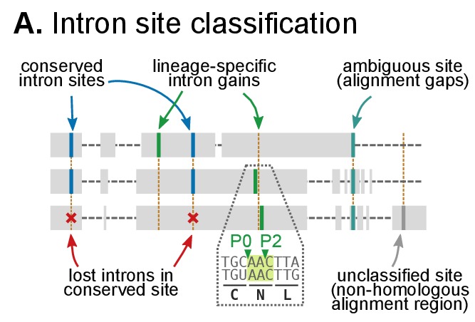
Figure 5—figure supplement 2. Phylogenetic distribution of the NMD machinery, SR splicing factors and RNA-binding domains in eukaryotes.

(A) Phylogenetic distribution of the NMD molecular toolkit across eukaryotes, as defined in Whelan et al. (2015), with a focus on unicellular holozoans and selected metazoans. The analysis includes 12 gene families: the core regulatory factors Upf1, Upf2 and Upf3 (also Smg2-4); the accessory proteins Smg1, Smg5/6/7 and Smg8/9; the release factors eRF1 and eRF3; and the exon junction complex (EJC) proteins eIF4A3, Y14, Magoh and MLN51. Extant species are color-coded by taxonomic assignment. Black dots indicate reconstructed LCAs within the line of descent between Metazoa and the LECA, whereas gray dots indicate LCAs not affiliated with Metaoza. Red, hollow circles indicate that a specific gene is absent from a given animal genome, but nevertheless present in a close relative in the same lineage (e.g., poriferans other than Amphimedon). See Methods for details on ortholog identification. Complete survey at the species level available as Figure 5—source data 3. Note that the core NMD tool-kit is conserved in most post-LECA LCAs, both in the animal and ichthyophonid ancestry. Secondary losses affect extant taxa: Corallochytrium lacks the complete EJC (only eIF4A3 is conserved) and homologs of Smg5/6/7 and Smg8/9. (B) Phylogenetic distribution of the SR splicing factors involved in alternative splicing determination across eukaryotes, as defined in Plass et al. (2008), with a focus on unicellular holozoans and selected metazoans. The analysis is focused on the following RNA-binding genes: SRP20/9G8 (human paralogs SRSF3/7), ASF (human paralogs SRSF1/9), SRP2 (human paralogs SRSF4/5/6), SRP1 (human paralogs SRSF2/8) and TRA2 (human paralogs TRA2A/B). Extant species are color-coded by taxonomic assignment. Black dots indicate reconstructed LCAs within the line of descent between Metazoa and the LECA, whereas gray dots indicate LCAs not affiliated with Metaoza. See Methods for details on ortholog identification. Complete survey at the species level available as Figure 5—source data 3. Note that the complement of SR genes is conserved in most post-LECA LCAs, including Opisthokonta, Holozoa and Metazoa. Secondary losses are, however, frequent in some lineages: SRSF1/9 is lost in Fungi, Teretosporea and Filasterea; Corallochytrium lacks all canonical SR genes but TRA2 and a fragmentary SRSF4/5/6; choanoflagellates have lost SRSF4/5/6, etc. (C) Counts of RNA-binding protein domains in extant eukaryotic genomes. Unicellular holozoans have a rich complement of RNA-binding proteins (domains per species: average 127.8; median 120), albeit less abundant than metazoans’ (domains per species: average 225.3; median 187).

DOI: http://dx.doi.org/10.7554/eLife.26036.023

Figure 5—figure supplement 3. Phylogenetic analysis of (A) eIF4A3, (B) Smg5/6/7, and (C) eRF3, using Maximum likelihood in IQ-TREE (supports are SH-like approximate likelihood ratio test/UFBS, respectively); including Bayesian inference supports for the ortologous groups of interest (BPP statistical supports, in red).

DOI: http://dx.doi.org/10.7554/eLife.26036.024