Figure 3.

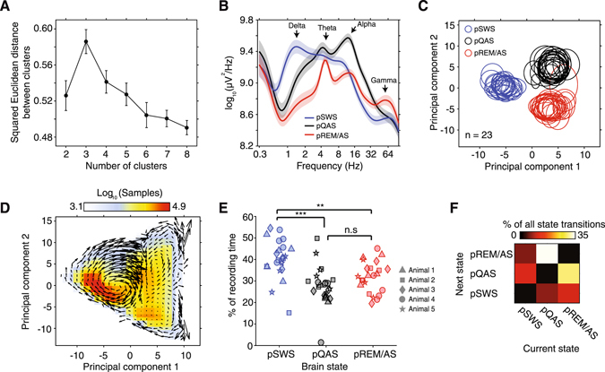
Objective classification of brain state by k-means clustering of data in state-space. (A) Data were clustered using a k-means clustering algorithm with the initial assumption of between 2 to 8 data clusters. Squared Euclidean distance between resultant clusters was maximal assuming 3 clusters, indicating that state/space data is optimally classified into 3 brain state clusters (error bars ± SEM). (B) The population average power spectrum computed across clustered brain states. Based on spectral characteristics of each state, clustered brain states were putatively labeled either presumed SWS (blue trace, slow wave sleep), quiet awake (black trace, pQAS), or rapid-eye-movement/active-state (red trace, pREM/AS). (C) The distribution of brain state data clusters across the first two principal components for all recording sessions and animals (n = 23). The mean of each cluster in state space is represented by the center of each ellipse, while standard deviation is represented by eccentricity along each axis. Note that brain states consistently localize in the same regions of state space across recordings and animals. (D) The number of samples binned across the first two components of state space provides a heat map of where animals spent the most time in state/space. Velocity vectors were overlaid to show the mean trajectories animals traversed through state space. (E) The percentage of time spent in each clustered sleep/wake state for each recording session. **p < 0.01, ***p < 0.001, kruskal-wallis test, Bonferroni corrected p-values. (F) The population average rate of transitions between brain states. Note that the most frequency state transitions occurred between pREM/AS and pQAS, which are maximally separated fluctuations along the second principal component axis.